It is strongly recommended to create a virtual environment that encapsulates your INDRA installation. Running the following commands will create a new environment and install INDRA into it. Replace /path/to/virtual/env with your desired location. This can be, e.g., ~/.virtualenvs/indra.
virtualenv -p python3 /path/to/virtual/env
source /path/to/virtual/env/bin/activate
pip install indra
pip uninstall -y enum34
deactivateThis package can be installed directly from GitHub by running the following commands in R:
if( !require(devtools) ) install.packages("devtools")
devtools::install_github("ArtemSokolov/indRa")The INDRA module is exposed through indra() function. It allows for direct access to any part of the INDRA API.
library( indRa )

## If using virtualenv
reticulate::use_virtualenv( "/path/to/virtual/env", required=TRUE )

## Access to INDRA is available through indra() function
indra()
# Module(indra)

## Reading a sentence with TRIPS
trips <- indra()$sources$trips
sentence <- 'MAP2K1 phosphorylates MAPK3 at Thr-202 and Tyr-204'
trips_processor <- trips$process_text( sentence )
trips_processor$statements
# [[1]]
# Phosphorylation(MAP2K1(), MAPK3(), T, 202)
#
# [[2]]
# Phosphorylation(MAP2K1(), MAPK3(), Y, 204)Extraneous output can be toggled through the Python logging mechanism
pyLogging <- reticulate::import( "logging" )
indra()$logger$setLevel( pyLogging$WARNING )The package provides additional functionality for constructing and manipulating interaction networks, based on statements retrieved from INDRA DB REST queries. A simple list of edges can be constructed through IDBquery(), which creates a data frame encapsulating the output of indra.sources.indra_db_rest.api.get_statements for all entities with HGNC mappings.
IDBquery( "SIK3" )
# # A tibble: 32 x 5
#   Hash               Activity        EvCnt Src   Trgt
#   <chr>              <chr>           <int> <chr> <chr>
# 1 7430532589474606   Phosphorylation     9 SIK3  PER2
# 2 -21145377478765295 Phosphorylation     8 SIK3  HDAC4
# 3 -260602555584320   Inhibition          4 SIK3  CRTC2
# 4 12365252834703035  Activation          3 SIK3  STK11
# 5 22779893853211724  Activation          3 SIK3  SIK3
# # … with 27 more rows

IDBquery( object="KLF4" )
# # A tibble: 621 x 5
#   Hash               Activity       EvCnt Src    Trgt
#   <chr>              <chr>          <int> <chr>  <chr>
# 1 34237034834082983  Activation        19 MIR145 KLF4
# 2 -1893896626253041  Acetylation       17 EP300  KLF4
# 3 -4171272971594532  IncreaseAmount    15 KLF4   KLF4
# 4 -2531422713809198  Activation        15 KLF4   KLF4
# 5 1490195882280611   Activation        15 STAT3  KLF4
# # … with 616 more rows
The package includes implementation of the Dijkstra's graph search algorithm for discovering paths between a source (e.g., a kinase) and downstream targets (e.g., transcription factors). The algorithm accepts an arbitrary path scoring function; by default, it uses lpgm (length-penalized geometric mean) provided with the package.
## Find paths from JAK2 to downstream Interferon TFs
PW <- dijkstra( "JAK2", trgts=c("NFKB1", "STAT1", "STAT2", "STAT3", "IRF1", "IRF3") )
# # A tibble: 7 x 3
#   Gene  Path             Score
#   <chr> <list>           <dbl>
# 1 STAT3 <tibble [1 × 4]>  5.56
# 2 STAT1 <tibble [1 × 4]>  4.56
# 3 STAT2 <tibble [1 × 4]>  2.20
# 4 NFKB1 <tibble [3 × 4]>  3.52
# 5 IRF1  <tibble [3 × 4]>  3.15
# 6 IRF3  <tibble [3 × 4]>  3.05

## Paths to individual targets can be retrieved from the Path column
P <- with(PW, setNames(Path, Gene))
P[["NFKB1"]]
# # A tibble: 3 x 4
#   Activity        EvCnt Src   Trgt
#   <chr>           <int> <chr> <chr>
# 1 Phosphorylation   261 JAK2  STAT3
# 2 Activation        329 STAT3 IL6
# 3 Activation         12 IL6   NFKB1
The search can be guided through the blacklist argument, which specifies which set of nodes should NOT be expanded. This guarantees that the final paths will not go through the blacklisted nodes. Note that blacklisting one or more targets does not prevent the algorithm from finding a path to them:
## STAT3 is both a target and blacklisted
PW2 <- dijkstra( "JAK2", c("NFKB1","IRF3","STAT3"), blacklist="STAT3" )
# # A tibble: 3 x 3
#   Gene  Path             Score
#   <chr> <list>           <dbl>
# 1 STAT3 <tibble [1 × 4]>  5.56
# 2 IRF3  <tibble [3 × 4]>  2.65
# 3 NFKB1 <tibble [3 × 4]>  2.65

## The path to NFKB1 no longer goes through STAT3
PW2$Path[[3]]
# # A tibble: 3 x 4
#   Activity        EvCnt Src   Trgt
#   <chr>           <int> <chr> <chr>
# 1 Phosphorylation    96 JAK2  STAT1
# 2 Activation        134 STAT1 IFNG
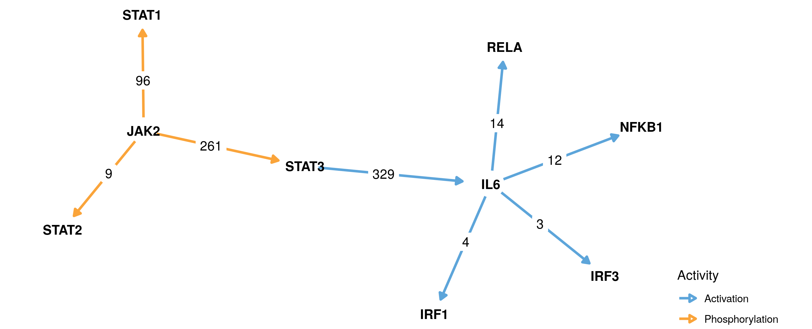
# 3 Activation 6 IFNG NFKB1The paths discovered through the graph search algorithms above can be visualized using plotPaths(). The function accepts one or more Path data frames discovered by, e.g., dijkstra() and returns a ggplot object that can be further modified using the standard grammar of graphics. Following the JAK2 example above, we may want to visualize the paths using our custom color scheme for the edges:
plotPaths( PW$Path ) + ggthemes::scale_color_few()