machine-learning-create-experiment.md

title	description	keywords	services	documentationcenter	author	manager	editor	ms.assetid	ms.service	ms.workload	ms.tgt_pltfrm	ms.devlang	ms.topic	ms.date	ms.author
A simple experiment in Machine Learning Studio | Microsoft Docs	This machine learning tutorial walks you through an easy data science experiment. We'll predict the price of a car using a regression algorithm.	experiment,linear regression,machine learning algorithms,machine learning tutorial,predictive modeling techniques,data science experiment	machine-learning		garyericson	jhubbard	cgronlun	b6176bb2-3bb6-4ebf-84d1-3598ee6e01c6	machine-learning	data-services	na	na	hero-article	12/14/2016	garye

Machine learning tutorial: Create your first data science experiment in Azure Machine Learning Studio

If you've never used Azure Machine Learning Studio before, this tutorial is for you.

In this tutorial, we'll walk through how to use Studio for the first time to create a machine learning experiment. The experiment will test an analytical model that predicts the price of an automobile based on different variables such as make and technical specifications.

Note

This tutorial shows you the basics of how to drag-and-drop modules onto your experiment, connect them together, run the experiment, and look at the results. We're not going to discuss the general topic of machine learning or how to select and use the 100+ built-in algorithms and data manipulation modules included in Studio.

If you're new to machine learning, the video series Data Science for Beginners might be a good place to start. This video series is a great introduction to machine learning using everyday language and concepts.

If you're familiar with machine learning, but you're looking for more general information about Machine Learning Studio, and the machine learning algorithms it contains, here are some good resources:

• What is Machine Learning Studio? - This is a high-level overview of Studio.
• Machine learning basics with algorithm examples - This infographic is useful if you want to learn more about the different types of machine learning algorithms included with Machine Learning Studio.
• Machine Learning Guide - This guide covers similar information as the infographic above, but in an interactive format.
• Machine learning algorithm cheat sheet and How to choose algorithms for Microsoft Azure Machine Learning - This downloadable poster and accompanying article discuss the Studio algorithms in depth.
• Machine Learning Studio: Algorithm and Module Help - This is the complete reference for all Studio modules, including machine learning algorithms,

[!INCLUDE machine-learning-free-trial]

How does Machine Learning Studio help?

Machine Learning Studio makes it easy to set up an experiment using drag-and-drop modules preprogrammed with predictive modeling techniques.

Using an interactive, visual workspace, you drag-and-drop datasets and analysis modules onto an interactive canvas. You connect them together to form an experiment that you run in Machine Learning Studio. You create a model, train the model, and score and test the model.

You can iterate on your model design, editing the experiment and running it until it gives you the results you're looking for. When your model is ready, you can publish it as a web service so that others can send it new data and get predictions in return.

Open Machine Learning Studio

To get started with Studio, go to https://studio.azureml.net. If you’ve signed into Machine Learning Studio before, click Sign In. Otherwise, click Sign up here and choose between free and paid options.

Sign in to Machine Learning Studio

Five steps to create an experiment

In this machine learning tutorial, you'll follow five basic steps to build an experiment in Machine Learning Studio to create, train, and score your model:

• Create a model
  • Step 1: Get data
  • Step 2: Prepare the data
  • Step 3: Define features
• Train the model
  • Step 4: Choose and apply a learning algorithm
• Score and test the model
  • Step 5: Predict new automobile prices

Tip

You can find a working copy of the following experiment in the Cortana Intelligence Gallery. Go to Your first data science experiment - Automobile price prediction and click Open in Studio to download a copy of the experiment into your Machine Learning Studio workspace.

Step 1: Get data

The first thing you need to perform machine learning is data. There are several sample datasets included with Machine Learning Studio that you can use, or you can import data from many sources. For this example, we'll use the sample dataset, Automobile price data (Raw), that's included in your workspace. This dataset includes entries for various individual automobiles, including information such as make, model, technical specifications, and price.

Here's how to get the dataset into your experiment.

1. Create a new experiment by clicking +NEW at the bottom of the Machine Learning Studio window, select EXPERIMENT, and then select Blank Experiment.

2. The experiment is given a default name that you can see at the top of the canvas. Select this text and rename it to something meaningful, for example, Automobile price prediction. The name doesn't need to be unique.

   

3. To the left of the experiment canvas is a palette of datasets and modules. Type automobile in the Search box at the top of this palette to find the dataset labeled Automobile price data (Raw). Drag this dataset to the experiment canvas.

   
   Find the automobile dataset and drag it onto the experiment canvas

To see what this data looks like, click the output port at the bottom of the automobile dataset, and then select Visualize.

Click the output port and select "Visualize"

Tip

Datasets and modules have input and output ports represented by small circles - input ports at the top, output ports at the bottom. To create a flow of data through your experiment, you'll connect an output port of one module to an input port of another. At any time, you can click the output port of a dataset or module to see what the data looks like at that point in the data flow.

In this sample dataset, each instance of an automobile appears as a row, and the variables associated with each automobile appear as columns. Given the variables for a specific automobile, we're going to try to predict the price in far-right column (column 26, titled "price").

View the automobile data in the data visualization window

Close the visualization window by clicking the "x" in the upper-right corner.

Step 2: Prepare the data

A dataset usually requires some preprocessing before it can be analyzed. For example, you might have noticed the missing values present in the columns of various rows. These missing values need to be cleaned so the model can analyze the data correctly. In our case, we'll remove any rows that have missing values. Also, the normalized-losses column has a large proportion of missing values, so we'll exclude that column from the model altogether.

Tip

Cleaning the missing values from input data is a prerequisite for using most of the modules.

First we add a module that removes the normalized-losses column completely, and then we add another module that removes any row that has missing data.

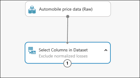
1. Type select columns in the Search box at the top of the module palette to find the Select Columns in Dataset module, then drag it to the experiment canvas. This module allows us to select which columns of data we want to include or exclude in the model.

2. Connect the output port of the Automobile price data (Raw) dataset to the input port of the Select Columns in Dataset module.

   
   Add the "Select Columns in Dataset" module to the experiment canvas and connect it

3. Click the Select Columns in Dataset module and click Launch column selector in the Properties pane.

   • On the left, click With rules
   • Under Begin With, click All columns. This directs Select Columns in Dataset to pass through all the columns (except those columns we're about to exclude).
   • From the drop-downs, select Exclude and column names, and then click inside the text box. A list of columns is displayed. Select normalized-losses, and it's added to the text box.
   • Click the check mark (OK) button to close the column selector (on the lower-right).

   
   Launch the column selector and exclude the "normalized-losses" column

   Now the properties pane for Select Columns in Dataset indicates that it will pass through all columns from the dataset except normalized-losses.

   
   The properties pane shows that the "normalized-losses" column is excluded

   [!TIP] You can add a comment to a module by double-clicking the module and entering text. This can help you see at a glance what the module is doing in your experiment. In this case, double-click the Select Columns in Dataset module and type the comment "Exclude normalized losses."

   
   Double-click a module to add a comment

4. Drag the Clean Missing Data module to the experiment canvas and connect it to the Select Columns in Dataset module. In the Properties pane, select Remove entire row under Cleaning mode. This directs Clean Missing Data to clean the data by removing rows that have any missing values. Double-click the module and type the comment "Remove missing value rows."

   
   Set the cleaning mode to "Remove entire row" for the "Clean Missing Data" module

5. Run the experiment by clicking RUN at the bottom of the page.

   When the experiment has finished running, all the modules have a green check mark to indicate that they finished successfully. Notice also the Finished running status in the upper-right corner.

After running it, the experiment should look something like this

Tip

Why did we run the experiment now? By running the experiment, the column definitions for our data pass from the dataset, through the Select Columns in Dataset module, and through the Clean Missing Data module. This means that any modules we connect to Clean Missing Data will also have this same information.

All we have done in the experiment up to this point is clean the data. If you want to view the cleaned dataset, click the left output port of the Clean Missing Data module and select Visualize. Notice that the normalized-losses column is no longer included, and there are no missing values.

Now that the data is clean, we're ready to specify what features we're going to use in the predictive model.

Step 3: Define features

In machine learning, features are individual measurable properties of something you’re interested in. In our dataset, each row represents one automobile, and each column is a feature of that automobile.

Finding a good set of features for creating a predictive model requires experimentation and knowledge about the problem you want to solve. Some features are better for predicting the target than others. Also, some features have a strong correlation with other features and can be removed. For example, city-mpg and highway-mpg are closely related so we can keep one and remove the other without significantly affecting the prediction.

Let's build a model that uses a subset of the features in our dataset. You can come back later and select different features, run the experiment again, and see if you get better results. But to start, let's try the following features:

make, body-style, wheel-base, engine-size, horsepower, peak-rpm, highway-mpg, price

1. Drag another Select Columns in Dataset module to the experiment canvas. Connect the left output port of the Clean Missing Data module to the input of the Select Columns in Dataset module.

   
   Connect the "Select Columns in Dataset" module to the "Clean Missing Data" module

2. Double-click the module and type "Select features for prediction."

3. Click Launch column selector in the Properties pane.

4. Click With rules.

5. Under Begin With, click No columns. In the filter row, select Include and column names and select our list of column names in the text box. This directs the module to not pass through any columns (features) except the ones that we specify.

6. Click the check mark (OK) button.

   
   Select the columns (features) to include in the prediction

This produces a filtered dataset containing only the features we want to pass to the learning algorithm we'll use in the next step. Later, you can return and try again with a different selection of features.

Step 4: Choose and apply a learning algorithm

Now that the data is ready, constructing a predictive model consists of training and testing. We'll use our data to train the model, and then we'll test the model to see how closely it's able to predict prices.

Classification and regression are two types of supervised machine learning algorithms. Classification predicts an answer from a defined set of categories, such as a color (red, blue, or green). Regression is used to predict a number.

Because we want to predict price, which is a number, we'll use a regression algorithm. For this example, we'll use a simple linear regression model.

Tip

If you want to learn more about different types of machine learning algorithms and when to use them, you might view the first video in the Data Science for Beginners series, The five questions data science answers. You might also look at the infographic Machine learning basics with algorithm examples, or check out the Machine learning algorithm cheat sheet.

We train the model by giving it a set of data that includes the price. The model scans the data and look for correlations between an automobile's features and its price. Then we'll test the model - we'll give it a set of features for automobiles we're familiar with and see how close the model comes to predicting the known price.

We'll use our data for both training the model and testing it by splitting the data into separate training and testing datasets.

1. Select and drag the Split Data module to the experiment canvas and connect it to the last Select Columns in Dataset module.

2. Click the Split Data module to select it. Find the Fraction of rows in the first output dataset (in the Properties pane to the right of the canvas) and set it to 0.75. This way, we'll use 75 percent of the data to train the model, and hold back 25 percent for testing (later, you can experiment with using different percentages).

   
   Set the split fraction of the "Split Data" module to 0.75

   [!TIP] By changing the Random seed parameter, you can produce different random samples for training and testing. This parameter controls the seeding of the pseudo-random number generator.

3. Run the experiment. When the experiment is run, the Select Columns in Dataset and Split Data modules pass column definitions to the modules we'll be adding next.

4. To select the learning algorithm, expand the Machine Learning category in the module palette to the left of the canvas, and then expand Initialize Model. This displays several categories of modules that can be used to initialize machine learning algorithms. For this experiment, select the Linear Regression module under the Regression category, and drag it to the experiment canvas. (You can also find the module by typing "linear regression" in the palette Search box.)

5. Find and drag the Train Model module to the experiment canvas. Connect the output of the Linear Regression module to the left input of the Train Model module, and connect the training data output (left port) of the Split Data module to the right input of the Train Model module.

   
   Connect the "Train Model" module to both the "Linear Regression" and "Split Data" modules

6. Click the Train Model module, click Launch column selector in the Properties pane, and then select the price column. This is the value that our model is going to predict.

   You select the price column in the column selector by moving it from the Available columns list to the Selected columns list.

   
   Select the price column for the "Train Model" module

7. Run the experiment.

We now have a trained regression model that can be used to score new automobile data to make price predictions.

After running, the experiment should now look something like this

Step 5: Predict new automobile prices

Now that we've trained the model using 75 percent of our data, we can use it to score the other 25 percent of the data to see how well our model functions.

1. Find and drag the Score Model module to the experiment canvas. Connect the output of the Train Model module to the left input port of Score Model. Connect the test data output (right port) of the Split Data module to the right input port of Score Model.

   
   Connect the "Score Model" module to both the "Train Model" and "Split Data" modules

2. Run the experiment and view the output from the Score Model module (click the output port of Score Model and select Visualize). The output shows the predicted values for price and the known values from the test data.

   
   Output of the "Score Model" module

3. Finally, we test the quality of the results. Select and drag the Evaluate Model module to the experiment canvas, and connect the output of the Score Model module to the left input of Evaluate Model.

   [!TIP] There are two input ports on the Evaluate Model module because it can be used to compare two models side by side. Later, you can add another algorithm to the experiment and use Evaluate Model to see which one gives better results.

4. Run the experiment.

To view the output from the Evaluate Model module, click the output port, and then select Visualize.

Evaluation results for the experiment

The following statistics are shown for our model:

• Mean Absolute Error (MAE): The average of absolute errors (an error is the difference between the predicted value and the actual value).
• Root Mean Squared Error (RMSE): The square root of the average of squared errors of predictions made on the test dataset.
• Relative Absolute Error: The average of absolute errors relative to the absolute difference between actual values and the average of all actual values.
• Relative Squared Error: The average of squared errors relative to the squared difference between the actual values and the average of all actual values.
• Coefficient of Determination: Also known as the R squared value, this is a statistical metric indicating how well a model fits the data.

For each of the error statistics, smaller is better. A smaller value indicates that the predictions more closely match the actual values. For Coefficient of Determination, the closer its value is to one (1.0), the better the predictions.

Final experiment

The final experiment should look something like this:

The final experiment

Next steps

Now that you've completed the first machine learning tutorial and have your experiment set up, you can continue to improve the model and then deploy it as a predictive web service.

• Iterate to try to improve the model - For example, you can change the features you use in your prediction. Or you can modify the properties of the Linear Regression algorithm or try a different algorithm altogether. You can even add multiple machine learning algorithms to your experiment at one time and compare two of them by using the Evaluate Model module. For an example of how to compare multiple models in a single experiment, see Compare Regressors in the Cortana Intelligence Gallery.

  [!TIP] To copy any iteration of your experiment, use the SAVE AS button at the bottom of the page. You can see all the iterations of your experiment by clicking VIEW RUN HISTORY at the bottom of the page. For more details, see Manage experiment iterations in Azure Machine Learning Studio.

• Deploy the model as a predictive web service - When you're satisfied with your model, you can deploy it as a web service to be used to predict automobile prices by using new data. For more details, see Deploy an Azure Machine Learning web service.

Want to learn more? For a more extensive and detailed walkthrough of the process of creating, training, scoring, and deploying a model, see Develop a predictive solution by using Azure Machine Learning.