PA1_template.md

Reproducible Research: Peer Assessment 1

Loading and preprocessing the data

First, let's load in a few libraries and read in the data.

if (!require(ggplot2)) {
    install.packages("ggplot2")
    library(ggplot2)
}

## Loading required package: ggplot2

if (!require(plyr)) {
    install.packages("plyr")
    library(plyr)
}

## Loading required package: plyr

if (!require(scales)) {
    install.packages("scales")
    library(scales)
}

## Loading required package: scales

data <- read.csv(unz("activity.zip", "activity.csv"))

What is mean total number of steps taken per day?

Let's plot the total number of steps per day:

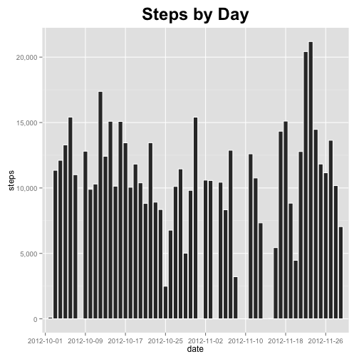
steps <- ddply(data, "date", summarise, steps = sum(steps, na.rm = TRUE))

ggplot(steps, aes(x = date, y = steps)) + geom_bar(stat = "identity", color = "white") + 
    scale_x_discrete(breaks = factor(steps$date)[seq(1, length(steps$date), 
        by = 8)]) + scale_y_continuous(labels = comma) + ggtitle("Steps by Day") + 
    theme(plot.title = element_text(size = rel(2), face = "bold", vjust = 1.5))

Let's find the mean and median per day:

stepMean <- mean(steps$steps)
stepMedian <- median(steps$steps)

The mean number of steps per day is 9354.2295. The median number of steps per day is 10395.

What is the average daily activity pattern?

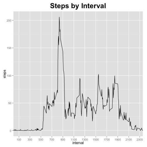
Let's plot the average number of steps per interval:

intervals <- ddply(data, "interval", summarise, steps = mean(steps, na.rm = TRUE))

ggplot(intervals, aes(x = interval, y = steps)) + geom_line(stat = "identity") + 
    scale_x_discrete(breaks = factor(seq(100, max(intervals$interval), by = 200))) + 
    scale_y_continuous(labels = comma) + ggtitle("Steps by Interval") + theme(plot.title = element_text(size = rel(2), 
    face = "bold", vjust = 1.5))

maxInt <- intervals[intervals$steps == max(intervals$steps), "interval"]

The interval with the maximum average number of daily steps is interval 835.

Imputing missing values

numMissing <- sum(is.na(data$steps))

There are 2304 missing values in the dataset.

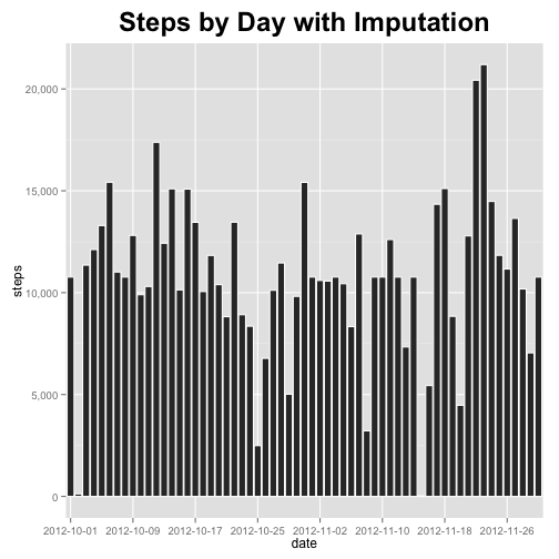
We will impute missing values with the average number of steps for that interval across all days, and then plot the resulting histogram.

data2 <- merge(data, rename(intervals, c(steps = "steps2")))
stepsNA <- which(is.na(data2$steps))
data2$steps[stepsNA] <- data2$steps2[stepsNA]

steps2 <- ddply(data2, "date", summarise, steps = sum(steps, na.rm = TRUE))

ggplot(steps2, aes(x = date, y = steps)) + geom_bar(stat = "identity", color = "white") + 
    scale_x_discrete(breaks = factor(steps2$date)[seq(1, length(steps2$date), 
        by = 8)]) + scale_y_continuous(labels = comma) + ggtitle("Steps by Day with Imputation") + 
    theme(plot.title = element_text(size = rel(2), face = "bold", vjust = 1.5))

Let's find the mean and median per day this time:

options(scipen = 999)
stepMean2 <- mean(steps2$steps)
stepMedian2 <- median(steps2$steps)

The new mean number of steps per day is 10766.1887.
The new median number of steps per day is 10766.1887.

Both of these values increased by imputing missing values with the average number of steps for that interval. These values are equal because a number of days consisted of nothing but missing values, which were then set to the mean of the other days' intervals. One such day then became the median day.

Unsurprisingly, there are more steps per day after imputing missing values.

Are there differences in activity patterns between weekdays and weekends?

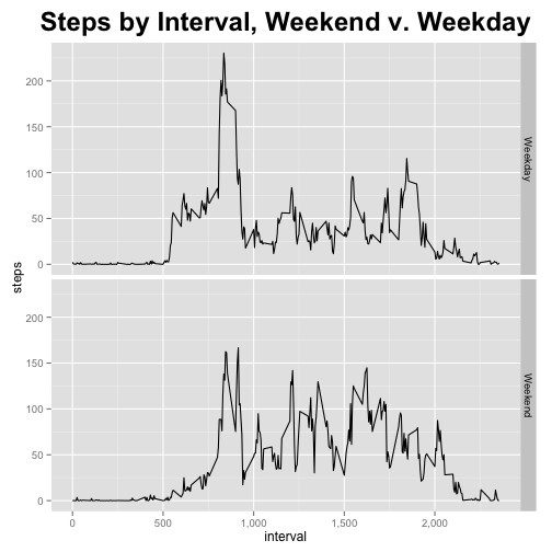
Let's plot the difference:

data2$weekdays <- factor(sapply(weekdays(as.Date(data2$date)), switch, Saturday = "Weekend", 
    Sunday = "Weekend", "Weekday"))

intervals2 <- ddply(data2, .(interval, weekdays), summarise, steps = mean(steps, 
    na.rm = TRUE))

ggplot(intervals2, aes(x = interval, y = steps)) + geom_line(stat = "identity") + 
    scale_x_continuous(labels = comma) + ggtitle("Steps by Interval, Weekend v. Weekday") + 
    theme(plot.title = element_text(size = rel(2), face = "bold", vjust = 1.5)) + 
    facet_grid(weekdays ~ .)