- and 2)
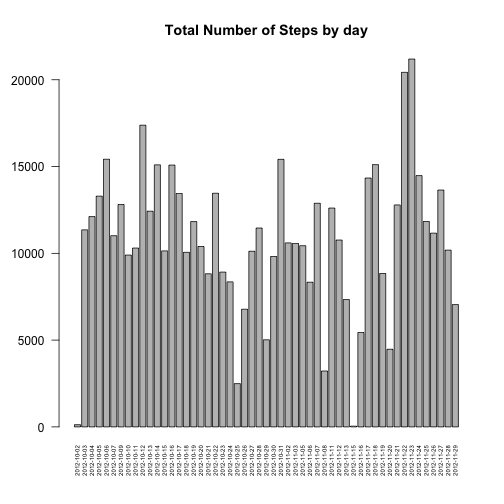
df <- read.table("~/activity.csv", sep = ",", header = TRUE, stringsAsFactors = FALSE)- Make a histogram of the total number of steps taken each day.
df1 <- aggregate(steps ~ date, data = df, na.rm = TRUE, sum)
with(df1, barplot(steps, main = "Total Number of Steps by day", ylab = "", xlab = "",
names = date, las = 2, cex.names = 0.5))- Calculate and report the mean and median total number of steps taken per day
df2 <- aggregate(steps ~ date, data = df, na.rm = TRUE, mean)
df3 <- aggregate(steps ~ date, data = df, na.rm = TRUE, median)
M <- merge(df2, df3, by = "date")
colnames(M) <- c("date", "mean", "median")
head(M)
## date mean median
## 1 2012-10-02 0.4375 0
## 2 2012-10-03 39.4167 0
## 3 2012-10-04 42.0694 0
## 4 2012-10-05 46.1597 0
## 5 2012-10-06 53.5417 0
## 6 2012-10-07 38.2465 0
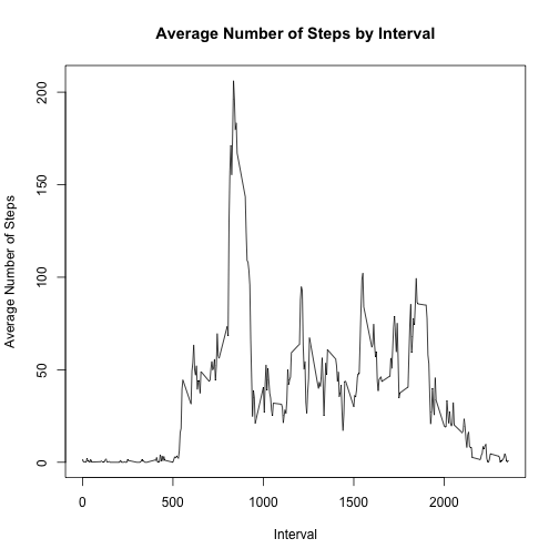
- Make a time series plot (i.e. type = "l") of the 5-minute interval (x-axis) and the average number of steps taken, averaged across all days (y-axis).
df4 <- aggregate(steps ~ interval, data = df, na.rm = TRUE, mean)
with(df4, plot(interval, steps, main = "Average Number of Steps by Interval",
ylab = "Average Number of Steps", xlab = "Interval", type = "l"))- Which 5-minute interval, on average across all the days in the dataset, contains the maximum number of steps?
df4[df4$steps == max(df4$steps), ]## interval steps
## 104 835 206.2
- Calculate and report the total number of missing values in the dataset (i.e. the total number of rows with NAs).
nrow(df[df$steps == "NA", ])## [1] 2304
- Devise a strategy for filling in all of the missing values in the dataset. The strategy does not need to be sophisticated. For example, you could use the mean/median for that day, or the mean for that 5-minute interval, etc.
Strategy: Mean for that 5-minute interval.
df <- read.table("~/activity.csv", sep = ",", header = TRUE, stringsAsFactors = FALSE)
df1 <- aggregate(steps ~ interval, data = df, na.rm = TRUE, mean)
t = nrow(df)/nrow(df1)
dfx = NULL
for (i in 1:t) {
    dfx <- rbind(dfx, df1)
}
for (i in 1:length(df)) {
    it = which(is.na(df$steps))
    for (j in 1:length(it)) {
        df$steps[it[j]] <- dfx$steps[it[j]]
    }
}
head(df)
## steps date interval
## 1 1.71698 2012-10-01 0
## 2 0.33962 2012-10-01 5
## 3 0.13208 2012-10-01 10
## 4 0.15094 2012-10-01 15
## 5 0.07547 2012-10-01 20
## 6 2.09434 2012-10-01 25
- Create a new dataset that is equal to the original dataset but with the missing data filled in.
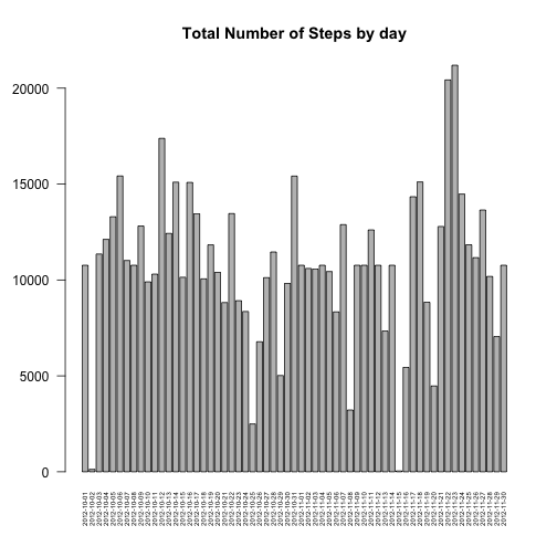
write.table(df, "activity1.csv", sep = ",", row.names = FALSE)- Make a histogram of the total number of steps taken each day and Calculate and report the mean and median total number of steps taken per day. Do these values differ from the estimates from the first part of the assignment? What is the impact of imputing missing data on the estimates of the total daily number of steps?
The impact is small, in general. Also it's possible to see that two days were added: 2012-10-01 and 2012-11-30. Moreover, the number of rows without NA is 17568 and the number of rows with NA is 2304. The total number of steps without NA is 570608 steps and the total number of steps with NA (filled in) is 656737.5 steps, ie. a difference of 89129.5 steps or +15%.
df1 <- aggregate(steps ~ date, data = df, na.rm = TRUE, sum)
with(df1, barplot(steps, main = "Total Number of Steps by day", ylab = "", xlab = "",
    names = date, las = 2, cex.names = 0.5))
df2 <- aggregate(steps ~ date, data = df, na.rm = TRUE, mean)
df3 <- aggregate(steps ~ date, data = df, na.rm = TRUE, median)
M <- merge(df2, df3, by = "date")
colnames(M) <- c("date", "mean", "median")
head(M)## date mean median
## 1 2012-10-01 37.3826 34.11
## 2 2012-10-02 0.4375 0.00
## 3 2012-10-03 39.4167 0.00
## 4 2012-10-04 42.0694 0.00
## 5 2012-10-05 46.1597 0.00
## 6 2012-10-06 53.5417 0.00
- Create a new factor variable in the dataset with two levels – “weekday” and “weekend” indicating whether a given date is a weekday or weekend day.
New factors: weekday and weekend
df$date <- as.Date(df$date)
df$day <- weekdays(df$date)
df$day[df$day == "Saturday" | df$day == "Sunday"] <- "weekend"
df$day[df$day != "weekend"] <- "weekday"
New table dft with new factors
dfwy <- subset(df, df$day == "weekday")
df4 <- aggregate(steps ~ interval, data = dfwy, na.rm = TRUE, mean)
df4$day <- "weekday"
dfwd <- subset(df, df$day == "weekend")
df5 <- aggregate(steps ~ interval, data = dfwd, na.rm = TRUE, mean)
df5$day <- "weekend"
dft <- rbind(df4, df5)
head(dft)
## interval steps day
## 1 0 2.25115 weekday
## 2 5 0.44528 weekday
## 3 10 0.17317 weekday
## 4 15 0.19790 weekday
## 5 20 0.09895 weekday
## 6 25 1.59036 weekday
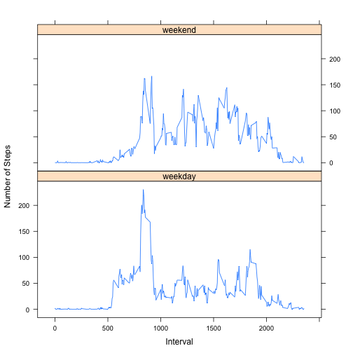
- Make a panel plot containing a time series plot (i.e. type = "l") of the 5-minute interval (x-axis) and the average number of steps taken, averaged across all weekday days or weekend days (y-axis).
library(lattice)
xyplot(dft$steps ~ dft$interval | dft$day, layout = c(1, 2), ylab = "Number of Steps",
    xlab = "Interval", type = "l")


