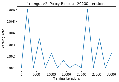
This repository includes a Keras callback to be used in training that allows implementation of cyclical learning rate policies, as detailed in Leslie Smith's paper Cyclical Learning Rates for Training Neural Networks arXiv:1506.01186v4.
A cyclical learning rate is a policy of learning rate adjustment that increases the learning rate off a base value in a cyclical nature. Typically the frequency of the cycle is constant, but the amplitude is often scaled dynamically at either each cycle or each mini-batch iteration.
The author demonstrates how CLR policies can provide quicker converge for some neural network tasks and architectures.
One example from the paper compares validation accuracy for classification on the CIFAR-10 dataset. In this specific example, the author used a triangular2 clr policy (detailed below). With clr, their model reached 81.4% validation accuracy in only 25,000 iterations compared to 70,000 iterations with standard hyperparameter settings.
One reason this approach may work well is because increasing the learning rate is an effective way of escaping saddle points. By cycling the learning rate, we're guaranteeing that such an increase will take place if we end up in a saddle point.
The purpose of this class is to not only provide an easy implementation of CLR for Keras, but to enable easy experimentation with policies not explored in the original paper.
clr_callback.py contains the callback class CyclicLR().
This class includes 3 built-in CLR policies, 'triangular', 'triangular2', and 'exp_range', as detailed in the original paper. It also allows for custom amplitude scaling functions, enabling easy experimentation.
Arguments for this class include:
base_lr: initial learning rate, which is the lower boundary in the cycle. This overrides optimizerlr. Default 0.001.max_lr: upper boundary in the cycle. Functionally, it defines the cycle amplitude (max_lr-base_lr). The lr at any cycle is the sum ofbase_lrand some scaling of the amplitude; thereforemax_lrmay not actually be reached depending on scaling function. Default 0.006.step_size: number of training iterations per half cycle. Authors suggest settingstep_size = (2-8) x (training iterations in epoch). Default 2000.mode: one of{'triangular', 'triangular2', 'exp_range'}. Values correspond to policies detailed below. Ifscale_fnis notNone, this argument is ignored. Default'triangular'.gamma: constant in'exp_range'scaling function,gamma^(cycle iterations). Default 1.scale_fn: Custom scaling policy defined by a single argument lambda function, where0 <= scale_fn(x) <= 1for allx >= 0.modeparameter is ignored when this argument is used. DefaultNone.scale_mode:{'cycle', 'iterations'}. Defines whetherscale_fnis evaluated on cycle number or cycle iterations (training iterations since start of cycle). Default is'cycle'.
NOTE: base_lr overrides optimizer.lr
The general structure of the policy algorithm is:
cycle = np.floor(1+iterations/(2*step_size))
x = np.abs(iterations/step_size - 2*cycle + 1)
lr= base_lr + (max_lr-base_lr)*np.maximum(0, (1-x))*scale_fn(x)
where x is either iterations or cycle, depending on scale_mode.
CyclicLR() can be used with any optimizer in Keras.
The author points out that the best accuracies are typically attained by ending with the base learning rate. Therefore it's recommended to make sure your training finishes at the end of the cycle.
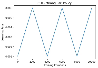
This method is a simple triangular cycle.
Basic algorithm:
cycle = np.floor(1+iterations/(2*step_size))
x = np.abs(iterations/step_size - 2*cycle + 1)
lr = base_lr + (max_lr-base_lr)*np.maximum(0, (1-x))
Default triangular clr policy example:
    clr = CyclicLR(base_lr=0.001, max_lr=0.006,
                        step_size=2000.)
    model.fit(X_train, Y_train, callbacks=[clr])
Results:
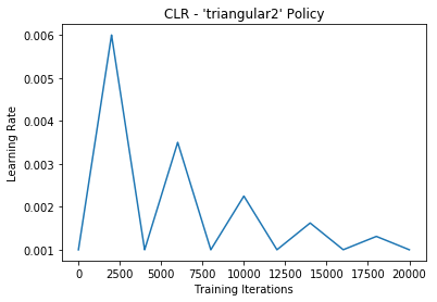
This method is a triangular cycle that decreases the cycle amplitude by half after each period, while keeping the base lr constant. This is an example of scaling on cycle number.
Basic algorithm:
cycle = np.floor(1+iterations/(2*step_size))
x = np.abs(iterations/step_size - 2*cycle + 1)
lr = base_lr + (max_lr-base_lr)*np.maximum(0, (1-x))/float(2**(cycle-1))
Default triangular clr policy example:
    clr = CyclicLR(base_lr=0.001, max_lr=0.006,
                        step_size=2000., mode='triangular2')
    model.fit(X_train, Y_train, callbacks=[clr])
Results:
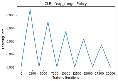
This method is a triangular cycle that scales the cycle amplitude by a factor gamma**(iterations), while keeping the base lr constant. This is an example of scaling on iteration.
Basic algorithm:
cycle = np.floor(1+iterations/(2*step_size))
x = np.abs(iterations/step_size - 2*cycle + 1)
lr= base_lr + (max_lr-base_lr)*np.maximum(0, (1-x))*gamma**(iterations)
Default triangular clr policy example:
    clr = CyclicLR(base_lr=0.001, max_lr=0.006,
                        step_size=2000., mode='exp_range',
                        gamma=0.99994)
    model.fit(X_train, Y_train, callbacks=[clr])
Results:
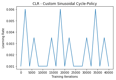
This method is a triangular cycle that scales the cycle amplitude sinusoidally. This is an example of scaling on cycle.
Basic algorithm:
cycle = np.floor(1+iterations/(2*step_size))
x = np.abs(iterations/step_size - 2*cycle + 1)
lr= base_lr + (max_lr-base_lr)*np.maximum(0, (1-x))*0.5*(1+np.sin(cycle*np.pi/2.))
Default custom cycle-policy example:
    clr_fn = lambda x: 0.5*(1+np.sin(x*np.pi/2.))
    clr = CyclicLR(base_lr=0.001, max_lr=0.006,
                        step_size=2000., scale_fn=clr_fn,
                        scale_mode='cycle')
    model.fit(X_train, Y_train, callbacks=[clr])
Results:
This method is a triangular cycle that scales the cycle amplitude as a function of the cycle iterations. This is an example of scaling on iteration.
Basic algorithm:
cycle = np.floor(1+iterations/(2*step_size))
x = np.abs(iterations/step_size - 2*cycle + 1)
lr= base_lr + (max_lr-base_lr)*np.maximum(0, (1-x))*1/(5**(iterations*0.0001))
Default custom cycle-policy example:
    clr_fn = lambda x: 1/(5**(x*0.0001))
    clr = CyclicLR(base_lr=0.001, max_lr=0.006,
                        step_size=2000., scale_fn=clr_fn,
                        scale_mode='iterations')
    model.fit(X_train, Y_train, callbacks=[clr])
Results:
This result highlights one of the key differences between scaling on cycle vs scaling on iteration. When you scale on cycle, the absolute change in learning rate from one iteration to the next is always constant in a cycle. Scaling on iteration alters the absolute change at every iteration; in this particular case, the absolute change is monotonically decreasing. This results in the curvature between peaks.
During training, you may wish to adjust your cycle parameters:
clr._reset(new_base_lr,
           new_max_lr,
           new_step_size)
Calling _reset() allows you to start a new cycle w/ new parameters.
_reset() also sets the cycle iteration count to zero. If you are using a policy with dynamic amplitude scaling, this ensures the scaling function is reset.
If an argument is not not included in the function call, then the corresponding parameter is unchanged in the new cycle. As a consequence, calling
clr._reset()simply resets the original cycle.
CyclicLR() keeps track of learning rates, loss, metrics and more in the history attribute dict. This generated many of the plots above.
Note: iterations in the history is the running training iterations; it is distinct from the cycle iterations and does not reset. This allows you to plot your learning rates over training iterations, even after you change/reset the cycle.
Example:
The author offers a simple approach to determining the boundaries of your cycle by increasing the learning rate over a number of epochs and observing the results. They refer to this as an "LR range test."
An LR range test can be done using the triangular policy; simply set base_lr and max_lr to define the entire range you wish to test over, and set step_size to be the total number of iterations in the number of epochs you wish to test on. This linearly increases the learning rate at each iteration over the range desired.
The author suggests choosing base_lr and max_lr by plotting accuracy vs. learning rate. Choose base_lr to be the learning rate where accuracy starts to increase, and choose max_lr to be the learning rate where accuracy starts to slow, oscillate, or fall (the elbow). In the example above, Smith chose 0.001 and 0.006 as base_lr and max_lr respectively.
In order to plot accuracy vs learning rate, you can use the .history attribute to get the learning rates and accuracy at each iteration.
model.fit(X, Y, callbacks=[clr])
h = clr.history
lr = h['lr']
acc = h['acc']Note that the clr callback updates the learning rate prior to any further learning rate adjustments as called for in a given optimizer.
clr_callback_tests.ipynb contains tests demonstrating desired behavior of optimizers.


