The latest version of dropClust is now available in desktop and online versions.
| Improved Interoperability | Integrative Analysis | Online web-server |
|---|---|---|
| SingleCellExperiment Container |  |
 |
Visit https://debsinha.shinyapps.io/dropClust/ for the online version.
The developer version of the R package can be installed with the following R commands:
library(devtools)
install_github("debsin/dropClust", dependencies = T, ref="devel")This vignette uses a small data set from the 10X website (3K PBMC dataset here ) to demonstrate a standard pipeline. This vignette can be used as a tutorial as well.
library(dropClust)
set.seed(0)dropClust loads UMI count expression data from three input files. The files follow the same structure as the datasets available from the 10X website, i.e.:
- count matrix file in sparse format
- transcriptome identifiers as a TSV file and
- gene identifiers as a TSV file
# Load Data, path contains decompressed files
sce <-readfiles(path = "C:/Projects/dropClust/data/pbmc3k/hg19/")dropClust performs pre-processing to remove poor quality cells and genes. dropClust is also equipped to mitigate batch-effects that may be present. The user does not need to provide any information regarding the source of the batch for individual transcriptomes. However, the batch-effect removal step is optional.
Cells are filtered based on the total UMI count in a cell specified by parameter min_count. Poor quality genes are removed based on the minimum number of cells min_count with expressions above a given threshold min_count.
# Filter poor quality cells.  A threshold th corresponds to the total count of a cell.
sce<-FilterCells(sce)
sce<-FilterGenes(sce)Count normalization is then performed with the good quality genes only. Normalized expression values is computed on the raw count data in a SingleCellExperiment object, using the median normalized total count.
sce<-CountNormalize(sce)
Further gene selection is carried out by ranking the genes based on its dispersion index.
# Select Top Dispersed Genes by setting ngenes_keep.
sce<-RankGenes(sce, ngenes_keep = 1000)Primary clustering is performed in a fast manner to estimate a gross structure of the data. Each of these clusters is then sampled to fine tune the clustering process.
sce<-Sampling(sce)
Another gene selection is performed to reduce the number of dimensions. PCA is used to identify genes affecting major components.
# Find PCA top 200 genes. This may take some time.
sce<-RankPCAGenes(sce)
By default best-fit, Louvain based clusters are returned. However, the user can tune the parameters to produce the desired number of clusters. The un-sampled transcriptomes are assigned cluster identifiers from among those identifiers produced from fine-tuning clustering. The post-hoc assignment can be controlled by setting the confidence value conf. High conf values will assign cluster identifiers to only those transcriptomes sharing a majority of common nearest neighbours.
# When `method = hclust`
# Adjust Minimum cluster size with argument minClusterSize (default = 20)
# Adjust tree cut with argument level deepSplit (default = 3), higher value produces more clusters.
sce<-Cluster(sce, method = "default", conf = 0.8)Compute 2D embeddings for samples followed by post-hoc clustering.
sce<-PlotEmbedding(sce, embedding = "umap", spread = 10, min_dist = 0.1)

plot_data = data.frame("Y1" = reducedDim(sce,"umap")[,1], Y2 = reducedDim(sce, "umap")[,2], color = sce$ClusterIDs)

ScatterPlot(plot_data,title = "Clusters")DE_genes_all = FindMarkers(sce, selected_clusters=NA, lfc_th = 1, q_th =0.001, nDE=30)
write.csv(DE_genes_all$genes,
file = file.path(tempdir(),"ct_genes.csv"),
quote = FALSE)
marker_genes = c("S100A8", "GNLY", "PF4")

p<-PlotMarkers(sce, marker_genes)# Draw heatmap
p<-PlotHeatmap(sce, DE_res = DE_genes_all$DE_res,nDE = 10)
print(p)Each dataset represents one batch and must be a SingleCellExperiment object. The objects are are merged by passing a list in the next step.
library(dropClust)
load(url("https://raw.githubusercontent.com/LuyiTian/CellBench_data/master/data/sincell_with_class.RData"))

objects = list()

objects[[1]] = sce_sc_10x_qc

objects[[2]] = sce_sc_CELseq2_qc

objects[[3]] = sce_sc_Dropseq_qcDatasets can be merged in two ways: using a set of DE genes from each batch or, using the union of the sets of highly variable genes from each batch.
set.seed(1)
dc.corr <-  Correction(merged_data,  method="default", close_th = 0.1, cells_th = 0.1,
components = 10, n_neighbors = 30, min_dist = 1)dc.corr = Cluster(dc.corr,method = "kmeans",centers = 3)
Compute 2D embeddings for samples followed by post-hoc clustering.
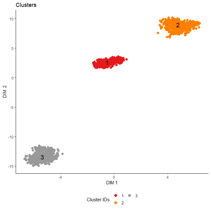
ScatterPlot(dc.corr, title = "Clusters")Users can use fastmnn method for batchcorrection. Specific arguments of fastmnn can also be passed through the Correction module.
merged_data.fastmnn<-Merge(all.objects,use.de.genes = FALSE)
set.seed(1)
mnn.corr <-  Correction(merged_data.fastmnn,  method="fastmnn", d = 10)
mnn.corr = Cluster(mnn.corr,method = "kmeans",centers = 3)
ScatterPlot(mnn.corr, title = "Clusters")de<-FindMarkers(dc.corr,q_th = 0.001, lfc_th = 1.2,nDE = 10)
de$genes.df


