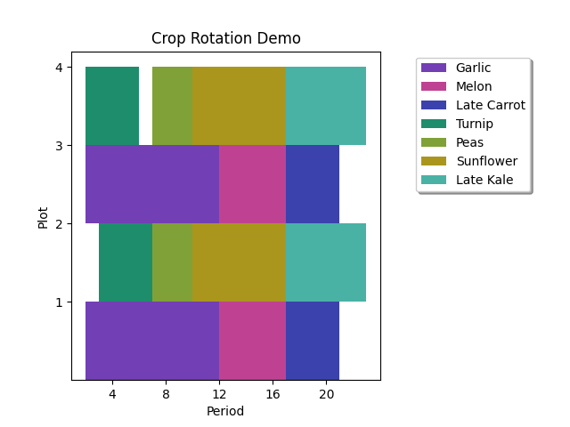
Crop rotation is the agricultural practice of growing a series of different crops in set of areas, called plots, over time. Crop rotation has benefits that include improved soil structure and reduced dependence on pesticides, herbicides, and fertilizers.
This example demonstrates a means of finding optimal crop rotations for a set of crops to be planted in a connected set of plots. This is done by formulating the problem as a discrete quadratic model (DQM) that can be solved using the D-Wave DQM solver.
To run the demo, type:
python crop_rotation.py
Note: the demo program will output an optimal crop rotation for a problem
instance defined by a problem file. By default, the demo program will use the
file data/problem1.yaml as problem file.
To solve a different problem instance, type:
python crop_rotation.py --path PATH_TO_PROBLEM_FILE
The program will produce an illustration of the solution such as this:
that will be saved as output.png.
We frame the problem of crop rotation as an optimization problem with the objective of maximizing plot utilization, subject to some constraints. This problem definition is based on the formulation described in Santos et al. (2008).
Crops are members of crop families. Each crop may be planted in any plot, and may be grown zero or more times in a rotation, but may be planted only in a certain season (defined as a range of time units). Each crop grows for a fixed amount of time before harvest. While a crop occupies a plot, no other crop may be planted in that plot.
Plots are connected, meaning each plot has zero or more adjacent plots. Adjacent plots may not have crops from the same family planted in them at the same time. Also, crops from the same family may not be planted sequentially in any plot.
These are the parameters of the problem:
M: number of time units in rotation periodL: number of plotsN: number of cropsN_f: number of crop familiesF_p: set of crops in crop family pS: set of pairs defining adjacent plotst_i: number of time units required between planting and harvest for crop iI_i: period of time [a, b] during which crop i can be planted
The decision variables for this problem are x_j,k. There are M * L of
these, one for each combination of time unit j and plot k. These are
discrete variables with up to N + 1 possible values. Assigning 0 to a
variable means no crop is planted in plot k at time j. The other values
i ∈ {1, ..., N}, assigned to x_j,k indicate that crop i is planted in
plot k at time j.
We can use binary variable x_i,j,k to indicate whether crop i (or no crop,
where i is 0) is assigned to discrete variable x_j,k.
When x_i,j,k is 1, crop i will occupy plot k from time j to time j + t_i.
The objective for the problem can now be written as:
The DQM solver solves minimization problems, so we change this to a minimization problem by negating the expression.
Now we need to consider our constraints. The first constraint is that two
crops cannot occupy the same space. Since our x_i,j,k variables indicate
planting, not occupation, we sum the x_i,j,k over each crop's grow time t_i
to represent occupation. This is actually a set of constraints; there are
M * L of them. They can be written as:
Our second constraint is that two crops from the same family cannot be planted
sequentially in the same plot. This is also a set of constraints; there are
N_f * M * L of them. They can be written as:
The third and final constraint is that two crops from the same family cannot be
planted at the same time in adjacent plots. This is also a set of constraints;
there are N_f * M * |S| of them. They can be written as:
Crop rotations are cyclic, so the period following M is 1. The second and
third constraints of the problem take wrapping into account. Here is an
illustration of a wrapping solution:
To formulate the crop rotation problem as a DQM, we want to choose linear and quadratic biases so that the solution energy will be at a minimum when utilization is maximized and the problem constraints are satisfied.
The DQM solver solves unconstrained problems, so we will use a
penalty parameter to
relate our constraints to our objective. We will use a single parameter,
gamma, as our constraints are equally important. We will choose a value for
gamma larger than the maximum change in the value of our objective that can
be obtained by changing one variable. This ensures that our constraints will
be satisfied. One such value is 1 + max(t_i).
Note that the DQM solver allows each variable to have a different number of
cases, or possible values. To reduce the total number of biases in the
problem, we will restrict the cases of the x_j,k variables to the set of
crops that can be planted in period j as defined by I_i.
The linear biases are the negated time values -t_i.
The quadratic, or interaction, biases arise from the constraints. As all of
our constraints are sums of variables that must equal either 0 or 1, we can use
a simple penalty scheme for each constraint. That is, we will add a positive
number (our penalty parameter, gamma) to the quadratic bias for every unique
pairing of the variables that appear in each constraint's sum.
To generate random problem instances for testing, type:
python problem_gen.py NROWS NCOLS
where NROWS and NCOLS provide the dimensions of a 2D plot grid. Additional parameters are described by:
python problem_gen.py --help
The random problem file will be written to stdout.
Santos, L. M. R. dos et al. "Crop rotation scheduling with adjacency constraints." Springer Science+Business Media, LLC, 26 Nov. 2008.
Released under the Apache License 2.0. See LICENSE file.


