README.md

Assignment 3

Setup

Environment setup

You can use the python environment you've set up for past assignments, or re-install it with our environment.yml file:

conda env create -f environment.yml
conda activate l3d

If you do not have Anaconda, you can quickly download it here, or via the command line in with:

wget https://repo.anaconda.com/miniconda/Miniconda3-latest-Linux-x86_64.sh
chmod +x Miniconda3-latest-Linux-x86_64.sh
bash Miniconda3-latest-Linux-x86_64.sh

Data

Most of the data for this assignment is provided in the github repo under data/. One of the assets (materials scene) is large, you need to download the zip file from https://drive.google.com/file/d/1v_0w1bx6m-SMZdqu3IFO71FEsu-VJJyb/view?usp=sharing and unzip it into data/ directory.

A. Neural Volume Rendering

0. Transmittance Calculation (10 points)

Transmittance calculation is a core part for the implementation of volume rendering. Your first task is to compute the transmittance of a ray going through a non-homogeneous medium (shown in the image below).
Please compute the transmittace in transmittance_calculation/a3_transmittance.pdf and submit the result on your assignment website. You can either hand write the result or edit the tex file and show a screenshot on your webpage, as long as it is readable by the TAs.

1. Differentiable Volume Rendering

In the emission-absorption (EA) model described in class, volumes are typically described by their appearance (e.g. emission) and geometry (absorption) at every point in 3D space. For part 1 of the assignment, you will implement a Differentiable Renderer for EA volumes, which you will use in parts 2 and 3. Differentiable renderers are extremely useful for 3D learning problems --- one reason is because they allow you to optimize scene parameters (i.e. perform inverse rendering) from image supervision only!

1.1. Familiarize yourself with the code structure

There are four major components of our differentiable volume rendering pipeline:

• The camera: pytorch3d.CameraBase
• The scene: SDFVolume in implicit.py
• The sampling routine: StratifiedSampler in sampler.py
• The renderer: VolumeRenderer in renderer.py

StratifiedSampler provides a method for sampling multiple points along a ray traveling through the scene (also known as raymarching). Together, a sampler and a renderer describe a rendering pipeline. Like traditional graphics pipelines, this rendering procedure is independent of the scene and camera.

The scene, sampler, and renderer are all packaged together under the Model class in volume_rendering_main.py. In particular the Model's forward method invokes a VolumeRenderer instance with a sampling strategy and volume as input.

Also, take a look at the RayBundle class in ray_utils.py, which provides a convenient wrapper around several inputs to the volume rendering procedure per ray.

1.2. Outline of tasks

In order to perform rendering, you will implement the following routines:

1. Ray sampling from cameras: you will fill out methods in ray_utils.py to generate world space rays from a particular camera.
2. Point sampling along rays: you will fill out the StratifiedSampler class to generate sample points along each world space ray
3. Rendering: you will fill out the VolumeRenderer class to evaluate a volume function at each sample point along a ray, and aggregate these evaluations to perform rendering.

1.3. Ray sampling (5 points)

Take a look at the render_images function in volume_rendering_main.py. It loops through a set of cameras, generates rays for each pixel on a camera, and renders these rays using a Model instance.

Implementation

Your first task is to implement:

1. get_pixels_from_image in ray_utils.py and
2. get_rays_from_pixels in ray_utils.py

which are used in render_images:

xy_grid = get_pixels_from_image(image_size, camera) # TODO: implement in ray_utils.py
ray_bundle = get_rays_from_pixels(xy_grid, camera) # TODO: implement in ray_utils.py

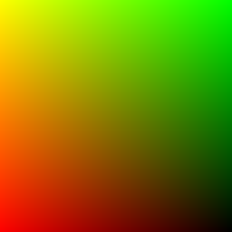
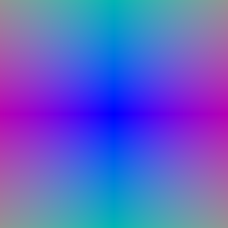
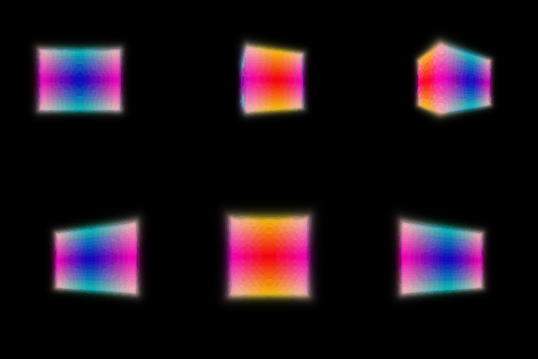
The get_pixels_from_image method generates pixel coordinates, ranging from [-1, 1] for each pixel in an image. The get_rays_from_pixels method generates rays for each pixel, by mapping from a camera's Normalized Device Coordinate (NDC) Space into world space.

Visualization

You can run the code for part 1 with:

# mkdir images (uncomment when running for the first time)
python volume_rendering_main.py --config-name=box

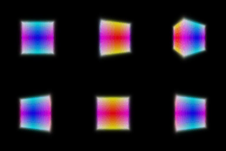
Once you have implemented these methods, verify that your output matches the TA output by visualizing both xy_grid and rays with the vis_grid and vis_rays functions in the render_images function in main.py. By default, the above command will crash and return an error. However, it should reach your visualization code before it does. The outputs of grid/ray visualization should look like this:

1.4. Point sampling (5 points)

Implementation

Your next task is to fill out StratifiedSampler in sampler.py. Implement the forward method, which:

1. Generates a set of distances between near and far and
2. Uses these distances to sample points offset from ray origins (RayBundle.origins) along ray directions (RayBundle.directions).
3. Stores the distances and sample points in RayBundle.sample_points and RayBundle.sample_lengths

Visualization

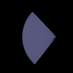
Once you have done this, use the render_points method in render_functions.py in order to visualize the point samples from the first camera. They should look like this:

1.5. Volume rendering (20 points)

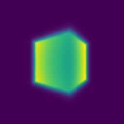
Finally, we can implement volume rendering! With the configs/box.yaml configuration, we provide you with an SDFVolume instance describing a box. You can check out the code for this function in implicit.py, which converts a signed distance function into a volume. If you want, you can even implement your own SDFVolume classes by creating new signed distance function class, and adding it to sdf_dict in implicit.py. Take a look at this great web page for formulas for some simple/complex SDFs.

Implementation

You will implement

1. VolumeRenderer._compute_weights and
2. VolumeRenderer._aggregate.
3. You will also modify the VolumeRenderer.forward method to render a depth map in addition to color from a volume

From each volume evaluation you will get both volume density, and a color:

# Call implicit function with sample points
implicit_output = implicit_fn(cur_ray_bundle)
density = implicit_output['density']
feature = implicit_output['feature']

You'll then use the following equation to render color along a ray:

where σ is density, Δt is the length of current ray segment, and L_e is color:

Compute the weights T * (1 - exp(-σ * Δt)) in VolumeRenderer._compute_weights, and perform the summation in VolumeRenderer._aggregate. Note that for the first segment T = 1.

Use weights, and aggregation function to render color and depth (stored in RayBundle.sample_lengths).

Visualization

By default, your results will be written out to images/part_1.gif. Provide a visualization of the depth in your write-up. Note that the depth should be normalized by its maximum value.

2. Optimizing a basic implicit volume

2.1. Random ray sampling (5 points)

Since you have now implemented a differentiable volume renderer, we can use it to optimize the parameters of a volume! We have provided a basic training loop in the train method in volume_rendering_main.py.

Depending on how many sample points we take for each ray, volume rendering can consume a lot of memory on the GPU (especially during the backward pass of gradient descent). Because of this, it usually makes sense to sample a subset of rays from a full image for each training iteration. In order to do this, implement the get_random_pixels_from_image method in ray_utils.py, invoked here:

xy_grid = get_random_pixels_from_image(cfg.training.batch_size, image_size, camera) # TODO: implement in ray_utils.py

2.2. Loss and training (5 points)

Replace the loss in train

loss = None

with mean squared error between the predicted colors and ground truth colors rgb_gt.

Once you've done this, you can run train a model with

python volume_rendering_main.py --config-name=train_box

This will optimize the position and side lengths of a box, given a few ground truth images with known camera poses (in the data folder). Report the center of the box, and the side lengths of the box after training, rounded to the nearest 1/100 decimal place.

2.3. Visualization

The code renders a spiral sequence of the optimized volume in images/part_2.gif. Compare this gif to the one below, and attach it in your write-up:

3. Optimizing a Neural Radiance Field (NeRF) (20 points)

In this part, you will implement an implicit volume as a Multi-Layer Perceptron (MLP) in the NeuraRadianceField class in implicit.py. This MLP should map 3D position to volume density and color. Specifically:

1. Your MLP should take in a RayBundle object in its forward method, and produce color and density for each sample point in the RayBundle.
2. You should also fill out the loss in train_nerf in the volume_rendering_main.py file.

You will then use this implicit volume to optimize a scene from a set of RGB images. We have implemented data loading, training, checkpointing for you, but this part will still require you to do a bit more legwork than for Parts 1 and 2. You will have to write the code for the MLP yourself --- feel free to reference the NeRF paper, though you should not directly copy code from an external repository.

Implementation

Here are a few things to note:

1. For now, your NeRF MLP does not need to handle view dependence, and can solely depend on 3D position.
2. You should use the ReLU activation to map the first network output to density (to ensure that density is non-negative)
3. You should use the Sigmoid activation to map the remaining raw network outputs to color
4. You can use Positional Encoding of the input to the network to achieve higher quality. We provide an implementation of positional encoding in the HarmonicEmbedding class in implicit.py.

Visualization

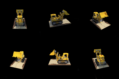
You can train a NeRF on the lego bulldozer dataset with

python volume_rendering_main.py --config-name=nerf_lego

This will create a NeRF with the NeuralRadianceField class in implicit.py, and use it as the implicit_fn in VolumeRenderer. It will also train a NeRF for 250 epochs on 128x128 images.

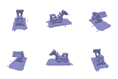
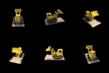
Feel free to modify the experimental settings in configs/nerf_lego.yaml --- though the current settings should allow you to train a NeRF on low-resolution inputs in a reasonable amount of time. After training, a spiral rendering will be written to images/part_3.gif. Report your results. It should look something like this:

4. NeRF Extras (CHOOSE ONE! More than one is extra credit)

4.1 View Dependence (10 pts)

Add view dependence to your NeRF model! Specifically, make it so that emission can vary with viewing direction. You can read NeRF or other papers for how to do this effectively --- if you're not careful, your network may overfit to the training images. Discuss the trade-offs between increased view dependence and generalization quality.

While you may use the lego scene to test your code, please employ the materials scene to show the results of your method on your webpage (experimental settings can be found in nerf_materials.yaml and nerf_materials_highres.yaml).

4.2 Coarse/Fine Sampling (10 pts)

NeRF employs two networks: a coarse network and a fine network. During the coarse pass, it uses the coarse network to get an estimate of geometry, and during fine pass uses these geometry estimates for better point sampling for the fine network. Implement this strategy and discuss trade-offs (speed / quality).

B. Neural Surface Rendering

5. Sphere Tracing (10pts)

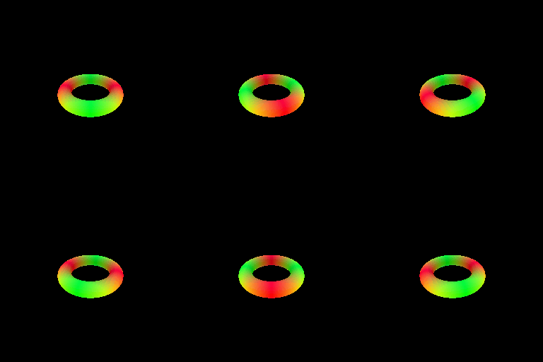
In this part you will implement sphere tracing for rendering an SDF, and use this implementation to render a simple torus. You will need to implement the sphere_tracing function in renderer.py. This function should return two outpus: (points, mask), where the points Tensor indicates the intersection point for each ray with the surface, and masks is a boolean Tensor indicating which rays intersected the surface.

You can run the code for part 5 with:

# mkdir images (uncomment when running for the first time)
python -m surface_rendering_main --config-name=torus_surface

This should save part_5.gif in the `images' folder. Please include this in your submission along with a short writeup describing your implementation.

6. Optimizing a Neural SDF (15pts)

In this part, you will implement an MLP architecture for a neural SDF, and train this neural SDF on point cloud data. You will do this by training the network to output a zero value at the observed points. To encourage the network to learn an SDF instead of an arbitrary function, we will use an 'eikonal' regularization which enforces the gradients of the predictions to behave in a certain way (search lecture slides for hints).

In this part you need to:

• Implement a MLP to predict distance: You should populate the NeuralSurface class in implicit.py. For this part, you need to define a MLP that helps you predict a distance for any input point. More concretely, you would need to define some MLP(s) in __init__ function, and use these to implement the get_distance function for this class. Hint: you can use a similar MLP to what you used to predict density in Part A, but remember that density and distance have different possible ranges!

• Implement Eikonal Constraint as a Loss: Define the eikonal_loss in losses.py.

After this, you should be able to train a NeuralSurface representation by:

python -m surface_rendering_main --config-name=points_surface

This should save save part_6_input.gif and part_6.gif in the images folder. The former visualizes the input point cloud used for training, and the latter shows your prediction which you should include on the webpage alongwith brief descriptions of your MLP and eikonal loss. You might need to tune hyperparameters (e.g. number of layers, epochs, weight of regularization, etc.) for good results.

7. VolSDF (15 pts)

In this part, you will implement a function converting SDF -> volume density and extend the NeuralSurface class to predict color.

• Color Prediction: Extend the the NeuralSurface class to predict per-point color. You may need to define a new MLP (a just a few new layers depending on how you implemented Q2). You should then implement the get_color and get_distance_color functions.

• SDF to Density: Read section 3.1 of the VolSDF Paper and implement their formula converting signed distance to density in the sdf_to_density function in renderer.py. In your write-up, give an intuitive explanation of what the parameters alpha and beta are doing here. Also, answer the following questions:

1. How does high beta bias your learned SDF? What about low beta?
2. Would an SDF be easier to train with volume rendering and low beta or high beta? Why?
3. Would you be more likely to learn an accurate surface with high beta or low beta? Why?

After implementing these, train an SDF on the lego bulldozer model with

python -m surface_rendering_main --config-name=volsdf_surface

This will save part_7_geometry.gif and part_7.gif. Experiment with hyper-parameters to and attach your best results on your webpage. Comment on the settings you chose, and why they seem to work well.

8. Neural Surface Extras (CHOOSE ONE! More than one is extra credit)

8.1. Render a Large Scene with Sphere Tracing (10 pts)

In Q5, you rendered a (lonely) Torus, but to the power of Sphere Tracing lies in the fact that it can render complex scenes efficiently. To observe this, try defining a ‘scene’ with many (> 20) primitives (e.g. Sphere, Torus, or another SDF from this website at different locations). See Lecture 2 for equations of what the ‘composed’ SDF of primitives is. You can then define a new class in implicit.py that instantiates a complex scene with many primitives, and modify the code for Q5 to render this scene instead of a simple torus.

8.2 Fewer Training Views (10 pts)

In Q7, we relied on 100 training views for a single scene. A benefit of using Surface representations, however, is that the geometry is better regularized and can in principle be inferred from fewer views. Experiment with using fewer training views (say 20) -- you can do this by changing train_idx in data laoder to use a smaller random subset of indices. You should also compare the VolSDF solution to a NeRF solution learned using similar views.

8.3 Alternate SDF to Density Conversions (10 pts)

In Q7, we used the equations from VolSDF Paper to convert SDF to density. You should try and compare alternate ways of doing this e.g. the ‘naive’ solution from the NeuS paper, or any other ways that you might want to propose!