For a short introduction to bacterial GWAS, you may wish to read this review.
This tutorial shows how to use pyseer to perform a GWAS for penicillin
resistance using 616 S. pneumoniae genomes collected from Massachusetts.
These genomes were first reported here and can be accessed
here. One of the earliest GWAS
studies in bacteria was performed using this data, and we will try to
replicate their results.
The data for this tutorial can be accessed here. Extract the archive:
tar xvf pyseer_tutorial.tar.bz2
To find the following files:
| File | Contents |
|---|---|
| assemblies.tar.bz2 | Archive of genome assemblies. |
| fsm_file_list.txt | Input to run fsm-lite. |
| snps.vcf.gz | SNPs mapped against the Spn23F reference. |
| gene_presence_absence.Rtab | Output from roary run on these genomes. |
| core_genome_aln.tree | IQ-TREE phylogeny (using -m GTR) from the core genome alignment. |
| resistances.pheno | Whether an isolate was resistant to penicillin, to be used as the phenotype. |
| mash_sketch.msh | mash sketch output, from running mash sketch -s 10000 -o mash_sketch *.fa. |
| Spn23F.fa | 23FSpn sequence. |
| Spn23F.gff | 23FSpn sequence and annotation. |
| 6952_7#3.fa | The draft sequence assembly of one isolate in the collection. |
| 6952_7#3.gff | The draft annotation of the isolate. |
Note
To run commands with the scripts/ directory you will need to have cloned the github repository (though other commands can continue to be run using your conda/pip install.
We will first of all demonstrate using pyseer with the original seer model,
using MDS components as fixed effects to control for the population structure.
We will test the association of SNPs mapped to a reference (provided as a VCF file) and COG
presence/absence (provided as and Rtab file, from running roary on the
annotations).
The first step is to estimate the population structure. We will do this using
a pairwise distance matrix produced using mash. Either create the mash
sketches yourself:
mkdir assemblies
cd assemblies
tar xf ../assemblies.tar.bz2
cd ..
mash sketch -s 10000 -o mash_sketch assemblies/*.fa
or use the pre-computed mash_sketch.msh directly. Next, use these to
calculate distances between all pairs of samples:
mash dist mash_sketch.msh mash_sketch.msh| square_mash > mash.tsv
Note
Alternatively, we could extract patristic distances from a phylogeny:
python scripts/phylogeny_distance.py core_genome_aln.tree > phylogeny_dists.tsv
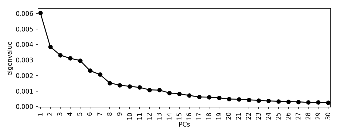
Let's perform an MDS and these distances and look at a scree plot to choose the number of dimensions to retain:
scree_plot_pyseer mash.tsv
There is a drop after about 8 dimensions, so we will use this many. This is subjective, and you may choose to include many more. This is a sensitivity/specificity tradeoff -- choosing more components is more likely to reduce false positives from population structure, at the expense of power. Using more components will also slightly increase computation time.
We can now run the analysis on the COGs:
pyseer --phenotypes resistances.pheno --pres gene_presence_absence.Rtab --distances mash.tsv --save-m mash_mds --max-dimensions 8 > penicillin_COGs.txt
Which prints the following to STDERR:
Read 603 phenotypes
Detected binary phenotype
Structure matrix has dimension (616, 616)
Analysing 603 samples found in both phenotype and structure matrix
10944 loaded variants
4857 filtered variants
6087 tested variants
6087 printed variants
pyseer has automatically matched the sample labels between the inputs, and
only used those which were present in the phenotype file. This has accounted
for the fact that not all of the samples were measured for the current
phenotype. We have used the default filters, so only intermediate frequency
COGs have been considered. The core genome COGs and low frequency COGs are in
the 4857 filtered out. Take a look at the top hits:
sort -g -k4,4 penicillin_COGs.txt | head

variant af      filter-pvalue   lrt-pvalue      beta    beta-std-err    intercept       PC1     PC2     PC3     PC4     PC5     PC6     PC7     PC8 notes
group_4276      7.79E-02        1.27E-11        2.70E-21        1.29E+01        7.12E-01        -1.29E+00       -7.01E-01       -2.75E+00       -6.64E+00    -9.02E-01       1.46E+01        -3.83E+00       -6.05E-01       -4.25E+00       high-bse
group_4417      8.96E-02        3.21E-09        4.72E-20        -6.08E+00       6.99E-01        -4.51E-01       -1.12E+00       5.08E-01        -5.61E+00    8.20E-01        8.19E+00        -4.95E-01       -4.53E-01       9.70E-01        bad-chisq
cpsG    1.18E-01        1.34E-16        1.69E-19        3.77E+00        5.25E-01        -1.34E+00       2.49E+00        1.24E-01        -5.19E+00   6.57E-01 1.01E+01        8.38E-02        -3.06E-01       8.48E-01
group_3096      1.18E-01        1.34E-16        1.69E-19        3.77E+00        5.25E-01        -1.34E+00       2.49E+00        1.24E-01        -5.19E+00    6.57E-01        1.01E+01        8.38E-02        -3.06E-01       8.48E-01
group_5738      1.18E-01        1.34E-16        1.69E-19        3.77E+00        5.25E-01        -1.34E+00       2.49E+00        1.24E-01        -5.19E+00    6.57E-01        1.01E+01        8.38E-02        -3.06E-01       8.48E-01
group_8161      1.18E-01        1.34E-16        1.69E-19        3.77E+00        5.25E-01        -1.34E+00       2.49E+00        1.24E-01        -5.19E+00    6.57E-01        1.01E+01        8.38E-02        -3.06E-01       8.48E-01
group_8834      1.18E-01        1.34E-16        1.69E-19        3.77E+00        5.25E-01        -1.34E+00       2.49E+00        1.24E-01        -5.19E+00    6.57E-01        1.01E+01        8.38E-02        -3.06E-01       8.48E-01
mnaA    1.18E-01        1.34E-16        1.69E-19        3.77E+00        5.25E-01        -1.34E+00       2.49E+00        1.24E-01        -5.19E+00   6.57E-01 1.01E+01        8.38E-02        -3.06E-01       8.48E-01
tagA    1.18E-01        1.34E-16        1.69E-19        3.77E+00        5.25E-01        -1.34E+00       2.49E+00        1.24E-01        -5.19E+00   6.57E-01 1.01E+01        8.38E-02        -3.06E-01       8.48E-01
Note that the first two rows have notes high-bse and bad-chisq
respectively. For the former this may represent a high effect size, low
frequency results. For the latter this is likely due to the MAF filter not
being stringent enough. The identical p-values of the other results are as these COGs
appear in exactly the same set of samples.
We will now perform an analysis using the SNPs produced from mapping reads
against the provided reference genome. To speed up the program we will load the
MDS decomposition mash_mds.pkl which was created by the COG analysis above:
pyseer --phenotypes resistances.pheno --vcf snps.vcf.gz --load-m mash_mds.pkl --lineage --print-samples > penicillin_SNPs.txt
This gives similar log messages:
Read 603 phenotypes
Detected binary phenotype
Loaded projection with dimension (603, 269)
Analysing 603 samples found in both phenotype and structure matrix
Writing lineage effects to lineage_effects.txt
198248 loaded variants
81370 filtered variants
116878 tested variants
116700 printed variants
We haven't specified the number of MDS dimensions to retain, so the default of
10 will be used (anything up to the 269 retained positive eigenvalues could be
chosen). Turning on the test for lineage effects with --lineage uses the
MDS components as the lineage, and writes the lineages most associated with
the phenotype to lineage_effects.txt:
lineage wald_test       p-value
MDS3    10.3041807281   0.0
MDS10   6.61332035523   3.75794950713e-11
MDS5    6.03559150525   1.58381441295e-09
MDS4    2.35736678835   0.0184050574981
MDS6    1.33118701438   0.183127483126
MDS2    1.02523510885   0.305252266
MDS9    0.850386297867  0.39511035157
MDS7    0.780676383001  0.434992854366
MDS1    0.478181602218  0.632520955891
MDS8    0.344928992152  0.730147754076
Variants associated with both the phenotype and MDS3, MDS10 or MDS5 may therefore be of interest as lineage effects.
The output now includes the lineage each variant is associated with, though not
all variants can be assigned a lineage. --print-samples forces the
inclusion of a comma separated list of samples the variant is present in
k-samples and not present in nk-samples (not shown here for brevity):
variant af      filter-pvalue   lrt-pvalue      beta    beta-std-err    intercept       PC1     PC2     PC3     PC4     PC5     PC6     PC7     PC8 PC9      PC10    lineage notes
26_23_G 4.31E-02        3.31E-01        4.42E-01        -4.19E-01       5.49E-01        -9.22E-01       1.84E-01        -6.00E-01       -7.53E+00   8.84E-01 2.05E+01        -1.79E+00       2.69E-01        1.16E-01        -7.52E-01       3.66E+00        MDS1
26_31_G_T       5.64E-02        3.94E-06        1.00E+00        6.78E-01        6.92E-01        -8.90E-01       1.97E-01        -4.13E-01       -7.05E+00    8.63E-01        1.91E+01        -1.33E+00       3.02E-01        9.13E-02        -4.99E-01       3.35E+00        MDS10   bad-chisq
26_83_A_G       4.58E-01        9.88E-04        3.25E-01        4.06E-01        4.13E-01        -1.21E+00       -1.43E-01       -7.84E-01       -7.35E+00    6.13E-01        1.91E+01        -1.19E+00       1.73E-01        6.44E-01        -4.47E-01       3.63E+00        MDS6
26_109_G_A      1.33E-02        1.46E-01        2.10E-14        4.15E+01        7.25E-01        -9.97E-01       9.39E-02        3.33E-02        -9.52E+00    1.72E+00        3.41E+01        1.38E+00        4.43E-01        -1.20E+00       6.82E-02        4.28E+00
26_184_G_A      3.32E-02        1.06E-02        8.49E-01        1.75E-01        9.11E-01        -9.65E-01       1.37E-01        -5.96E-01       -7.42E+00    8.65E-01        1.98E+01        -1.71E+00       3.00E-01        2.78E-01        -6.18E-01       3.63E+00
26_281_C_T      1.01E-01        1.20E-05        3.97E-01        -5.91E-01       6.91E-01        -9.08E-01       1.12E-01        -7.04E-01       -7.24E+00    7.18E-01        2.02E+01        -1.73E+00       4.32E-01        3.50E-01        -6.84E-01       3.69E+00        MDS4
26_293_G_A      1.49E-02        3.50E-01        5.31E-01        7.06E-01        1.07E+00        -9.73E-01       1.29E-01        -6.11E-01       -7.49E+00    9.16E-01        2.03E+01        -1.54E+00       3.02E-01        2.55E-01        -5.93E-01       3.66E+00        MDS6
26_483_G_A      2.37E-01        7.85E-02        1.82E-02        9.16E-01        3.90E-01        -1.32E+00       -2.83E-01       -1.30E+00       -7.28E+00    6.77E-01        1.78E+01        -1.79E+00       2.59E-01        1.10E+00        3.15E-02        3.44E+00        MDS9
26_539_G_A      1.33E-02        1.46E-01        2.10E-14        4.15E+01        7.25E-01        -9.97E-01       9.39E-02        3.33E-02        -9.52E+00    1.72E+00        3.41E+01        1.38E+00        4.43E-01        -1.20E+00       6.82E-02        4.28E+00
This contains co-ordinates and p-values, which can be converted to a .plot
file using the following awk one-liner:
cat <(echo "#CHR SNP BP minLOG10(P) log10(p) r^2") \\
<(paste <(sed '1d' penicillin_SNPs.txt | cut -d "_" -f 2) \\
<(sed '1d' penicillin_SNPs.txt | cut -f 4) | \\
awk '{p = -log($2)/log(10); print "26",".",$1,p,p,"0"}' ) | \\
tr ' ' '\t' > penicillin_snps.plot
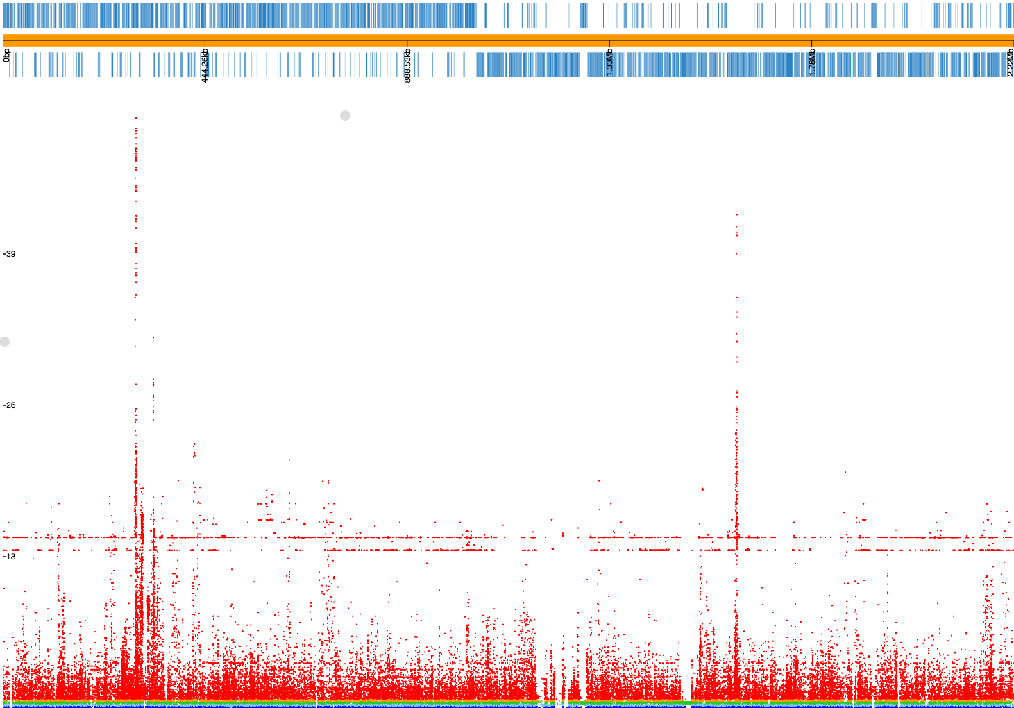
If we drag and drop 23FSpn.gff and penicillin_snps.plot files into
phandango you should see
a Manhattan plot similar to this:
The three highest peaks are in the pbp2x, pbp1a and pbp2b genes,
which are the correct loci. There are also flat lines, suggesting
these may be lineage effects from population structure that has not been fully
controlled for. In actual fact, if we inspect the SNPs along these two lines
(p = 2.10E-14 and p = 1.58E-15) we see that all of them are annotated
with the note bad-chisq and are at the lower end of the included minor allele
frequency threshold (1.3% and 1.2% respectively). These are therefore variants
which were underpowered, and the associations are spurious. They should be
filtered out, and we should probably have used a MAF cutoff of at least 2%
given the total number of samples we have. As a rule of thumb, a MAF cutoff
corresponding to a MAC of at least 10 isn't a bad start. Let's run it again:
pyseer --phenotypes resistances.pheno --vcf snps.vcf.gz --load-m output/mash_mds.pkl --min-af 0.02 --max-af 0.98 > penicillin_SNPs.txt

Read 603 phenotypes
Detected binary phenotype
Loaded projection with dimension (603, 269)
Analysing 603 samples found in both phenotype and structure matrix
198248 loaded variants
106949 filtered variants
91299 tested variants
91225 printed variants
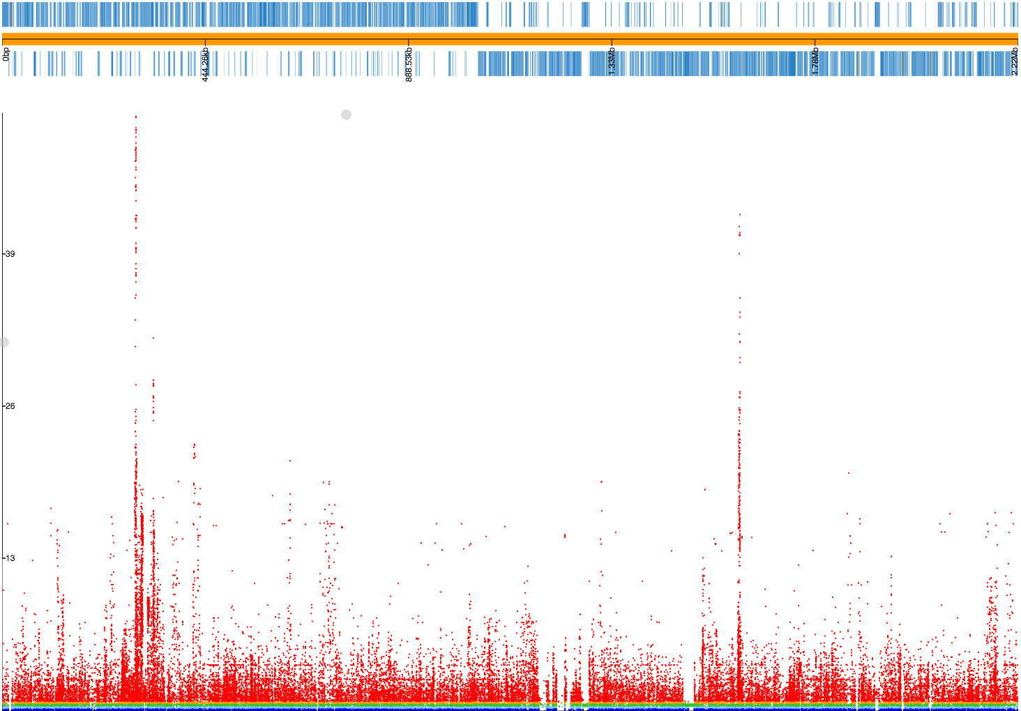
A lot more low frequency variants have been filtered out this time, and if we make a plot file our Manhattan plot looks much cleaner:
We will now use k-mers as a variant to test both short variation as well as
gene presence/absence. This can be done using the steps above replacing the
--vcf argument with --kmers, which would replicate the results from the
original seer tutorial. For demonstration purposes we will instead use the
other association model available in pyseer, the linear mixed model.
First, count the k-mers from the assemblies:
mkdir -p assemblies
cd assemblies
tar xvf ../assemblies.tar.bz2
fsm-lite -l ../fsm_file_list.txt -s 6 -S 610 -v -t fsm_kmers | gzip -c - > ../fsm_kmers.txt.gz
cd ..
This will require you to have fsm-lite installed If you do not have the time/resources to do this, you can follow the rest of these steps using the SNPs as above.
Note
Everything here also applies to unitigs, which can be called with unitig-counter. These are generally recommended due to their lower redundancy (and are also therefore faster) and potentially easier interpretation.
To correct for population structure we must supply pyseer with the kinship
matrix K using the --similarities argument (or --load-lmm if using
a previous analysis where --save-lmm was used).
We will use the distances from the core genome phylogeny, which has been midpointed rooted:
python scripts/phylogeny_distance.py --lmm core_genome_aln.tree > phylogeny_K.tsv
Note
Alternatively, we could extract a kinship matrix from the mapped SNPs by calculating K = GG^T
similarity_pyseer --vcf snps.vcf.gz samples.txt > gg.snps.txt
We can now run pyseer with --lmm. Due to the large number of k-mers we are going to test, we will increase the
number of CPUs used to 8:
pyseer --lmm --phenotypes resistances.pheno --kmers fsm_kmers.txt.gz --similarity phylogeny_K.tsv --output-patterns kmer_patterns.txt --cpu 8 > penicillin_kmers.txt
The heritability h^2 estimated from the kinship matrix K is printed to STDERR, and after about 5 hours the results have finished being written:
Read 603 phenotypes
Detected binary phenotype
Setting up LMM
Similarity matrix has dimension (616, 616)
Analysing 603 samples found in both phenotype and similarity matrix
h^2 = 0.90
15167239 loaded variants
1042215 filtered variants
14125024 tested variants
14124993 printed variants
Note
The heritability estimate shouldn't be interpreted as a quantitative measure for this binary phenotype, but a high heritability is consistent with the mechanism of penicillin resistance in this species (the sequence can give up to 99% prediction accuracy of penicillin resistance).
The results look similar, though also include the heritability of each variant tested:
variant af      filter-pvalue   lrt-pvalue      beta    beta-std-err    variant_h2      notes
TTTTTTTTTTTT    8.11E-01        1.51E-06        1.05E-01        6.13E-02        3.78E-02        6.60E-02
TTTTTTTTTTTTT   7.08E-01        6.20E-06        4.03E-01        -3.34E-02       3.98E-02        3.41E-02
TTTTTTTTTTTTTT  5.97E-01        6.39E-05        1.81E-01        -4.05E-02       3.03E-02        5.45E-02
TTTTTTTTTTTTTTT 3.55E-01        5.92E-04        7.90E-01        -6.84E-03       2.57E-02        1.09E-02
TTTTTTTTTTTTTTTT        1.48E-01        2.11E-03        7.38E-01        1.13E-02        3.37E-02        1.37E-02
TTTTTTTTTTTTTTTTT       6.47E-02        3.94E-01        4.89E-01        3.11E-02        4.49E-02        2.83E-02
TTTTTTTTTTTTTTTTTT      3.48E-02        2.73E-02        2.59E-01        -6.73E-02       5.96E-02        4.60E-02
TTTTTTTTTTTTTTTTTTT     2.32E-02        2.18E-01        6.96E-01        -2.81E-02       7.19E-02        1.59E-02
TTTTTTTTTTTTTTTTTTTT    1.66E-02        2.58E-01        9.46E-01        -5.63E-03       8.37E-02        2.74E-03
The downstream processing of the k-mer results in penicillin_kmers.txt will be
shown in the next section. Before that, we can determine a significance threshold
using the number of unique k-mer patterns:
python scripts/count_patterns.py kmer_patterns.txt
Patterns:       2627332
Threshold:      1.90E-08
This is over five times lower than the total number of k-mers tested, so stops us from being hyper-conservative with the multiple testing correction.
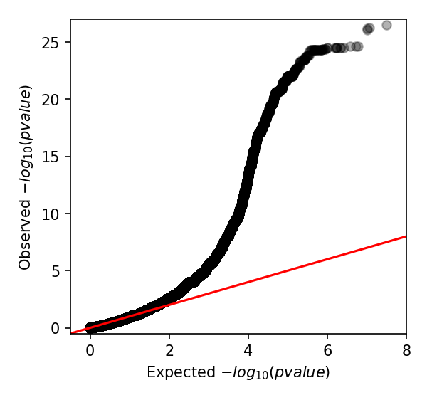
We can also create a Q-Q plot to check that p-values are not inflated. We can do that
by using the qq_plot.py script:
python scripts/qq_plot.py penicillin_kmers.txt
which produces the following Q-Q plot:
When interpreting this plot, check that it is well controlled at low p-values and doesn't show any large 'shelves' symptomatic of poorly controlled confounding population structure. Although this plot is far above the null (as indeed, there are many k-mers associated with penicillin resistance), the p-values up to 0.01 are as expected which is what we're after.
For the final step we will work with only those k-mers which exceeded the
significance threshold in the mixed model analysis. We will filter these from
the output using a simple awk command:
cat <(head -1 penicillin_kmers.txt) <(awk '$4<1.90E-08 {print $0}' penicillin_kmers.txt) > significant_kmers.txt
There are 5327 significant k-mers.
Let's use bwa mem to map these to
the reference provided:
phandango_mapper significant_kmers.txt Spn23F.fa Spn23F_kmers.plot

Read 5327 k-mers
Mapped 2425 k-mers
Not all the k-mers have been mapped, which is usually the case. Note there are 2459 mapping lines in the output, as 34 secondary mappings we included. It is a good idea to map to range of references to help with an interpretion for all of the significant k-mers. The k-mer annotation step, described next, also helps cover all k-mers. Let's look at the plot file in phandango:
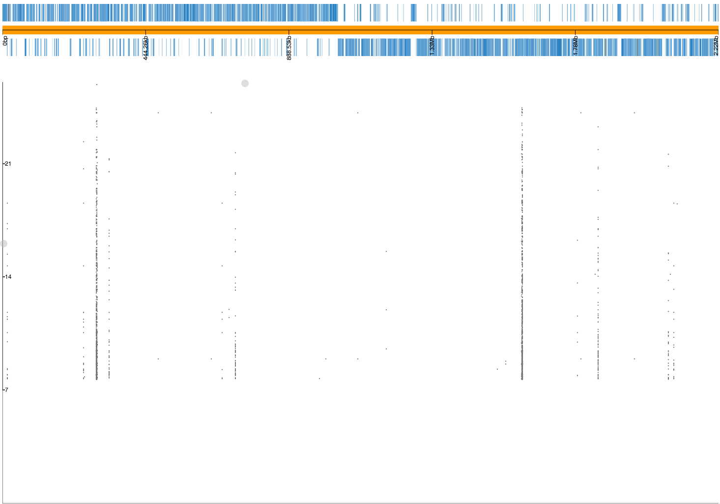
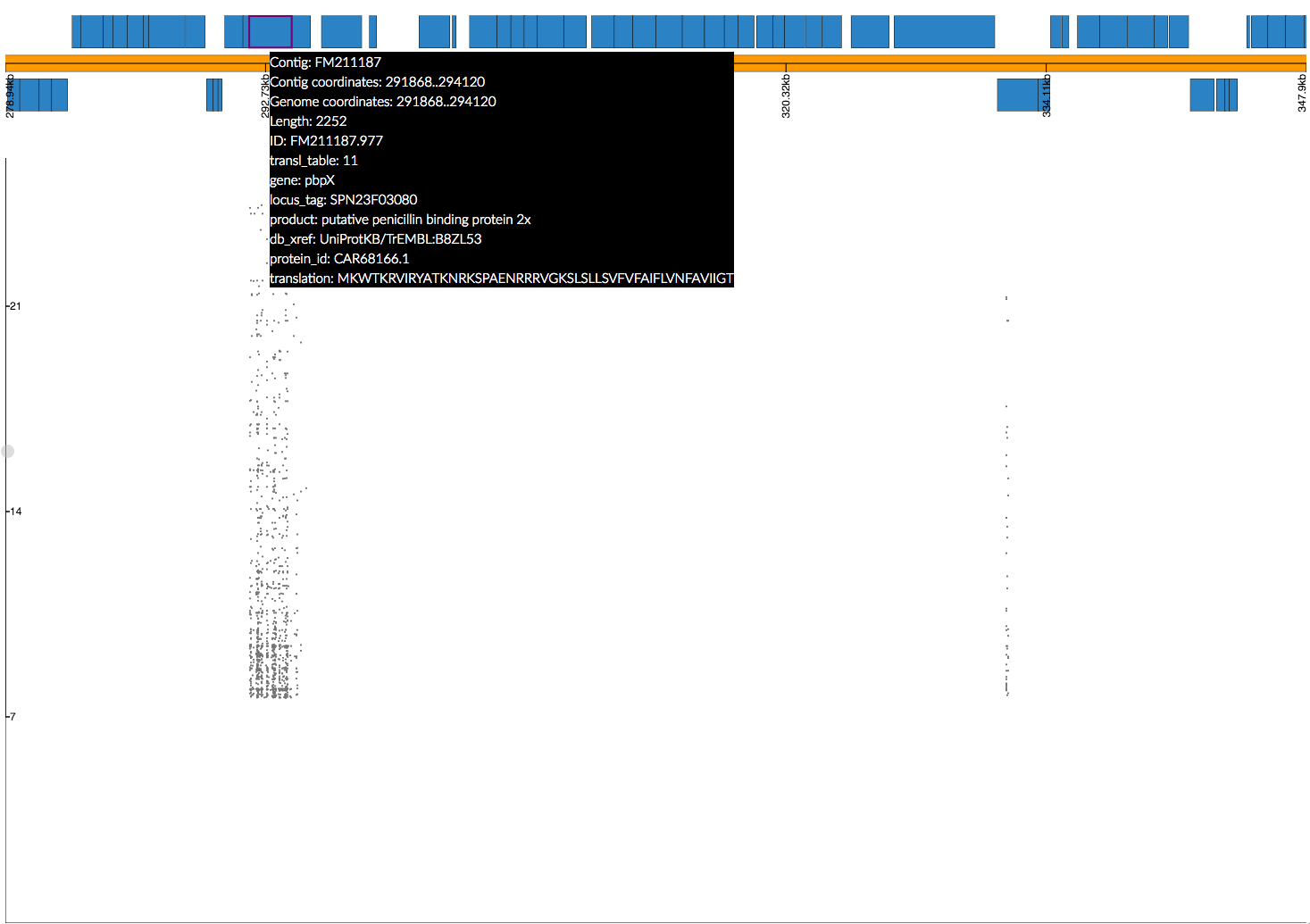
In this view we no longer see all of the Manhattan plot as we have filtered out the low p-value k-mers. There is generally less noise due to LD/population structure when compared to our previous result above. There are peaks in the three pbp genes again, with the strongest results in pbp2x and pbp2b as before. Zooming in:
The whole pbp2x gene is covered by significant k-mers, whereas only a small part of pbp1a is hit. This could be due to the fact that only some sites in pbp1a can be variable, only some of the variable sites affect penicllin resistance, or due to the ability to map k-mers to this region.
We can annotate these k-mers with the genes they are found in, or are near. To try and map every k-mer we can include a number of different reference annotations, as well as all the draft annotations of the sequences the k-mers were counted from. For the purposes of this tutorial we will demonstrate with a single type of each annotation, but this could be expanded by adding all the annotated assemblies to the input.
We'll start by creating a references.txt file listing the annotations we
wish to use (see :ref:`annotate-kmers` for more information on how to construct
this file):
Spn23F.fa    Spn23F.gff      ref
6952_7#3.fa  6952_7#3.gff    draft
Now run the script. This will iterate down the list of annotations, annotating the k-mers which
haven't already been mapped to a previous annotation (requires bedtools, bedops and the
pybedtools package):
annotate_hits_pyseer significant_kmers.txt references.txt annotated_kmers.txt

Reference 1
5327 kmers remain
Draft reference 2
2902 kmers remain
Note
If this runs slowly you can split the significant_kmers.txt file into
pieces to parallelise the process.
Note
By default annotate_hits_pyseer will only consider CDS features in the
provided GFF files. If you want to consider other feature types you can use the
--feature-type option (e.g. --feature-type rRNA --feature-type tRNA).
Annotations marked ref can partially match between k-mer and reference
sequence, whereas those marked draft require an exact match. In this case
the single draft didn't add any matches.
The genes a k-mer is in, as well as the nearest upstream and downstream are added to the
output:
TTTTTTTCTACAATAAAATAGGCTCCATAATATCTATAGTGGATTTACCCACTACAAATATTATAGAACCCGTTTTATTATGGAAAGACTTATTGGACTT    6.47E-02        2.08E-12        2.10E-09        7.97E-01        1.31E-01        2.41E-01        FM211187:252213-252312;FM211187.832;;FM211187.834
TTTTTTTATAGATTTCAGGATCAGCCAAATAGTAATCCG 8.42E-01        1.03E-36        2.99E-10        -4.38E-01       6.83E-02        2.53E-01        FM211187:723388-723417;FM211187.2367;;FM211187.2371
TTTTTTTATAGATTTCAGGATCAGCCAAATAGTAATCCGCCAGCTGGCGTT     8.39E-01        3.38E-35        4.04E-09        -3.95E-01       6.62E-02        2.37E-01        FM211187:1614084-1614122;penA;penA;penA
The output format is contig:position;upstream;in;downstream.
The first line shows the k-mer was mapped to FM211187:252213-252312, the
nearest gene downstream having ID FM211187.832 and upstream having ID FM211187.834.
The third line shows that k-mer overlaps penA -- note when a gene= field
is found this is used in preference to the ID= field.
Finally, we can summarise these annotations to create a plot of significant
genes. We will only use genes k-mers are actually in, but if we wanted to we
could also include up/downstream genes by using the --nearby option:
python scripts/summarise_annotations.py annotated_kmers.txt > gene_hits.txt
We'll use ggplot2 in R to plot these results:
require(ggplot2)
require(ggrepel)
library(ggrepel)

gene_hits = read.table("gene_hits.txt", stringsAsFactors=FALSE, header=TRUE)

ggplot(gene_hits, aes(x=avg_beta, y=maxp, colour=avg_maf, size=hits, label=gene)) +
   geom_point(alpha=0.5) +
   geom_text_repel(aes(size=60), show.legend = FALSE, colour='black') +
   scale_size("Number of k-mers", range=c(1,10)) +
   scale_colour_gradient('Average MAF') +
   theme_bw(base_size=14) +
   ggtitle("Penicillin resistance") +
   xlab("Average effect size") +
   ylab("Maximum -log10(p-value)")
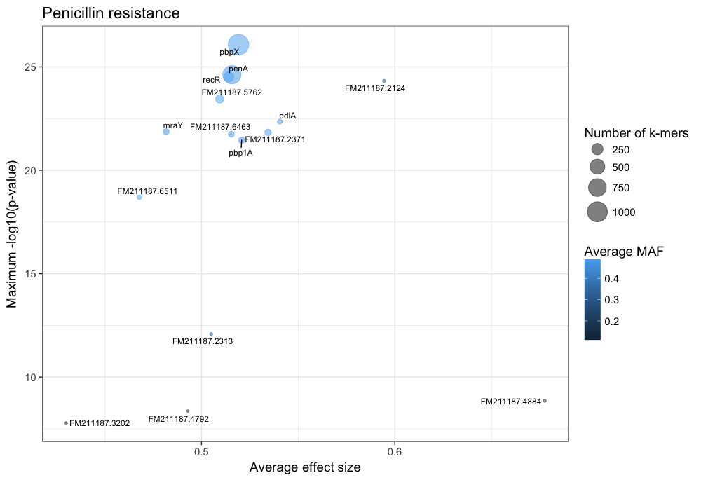
You can customise this however you wish (for example adding the customary italics on gene names); these commands will produce a plot like this:
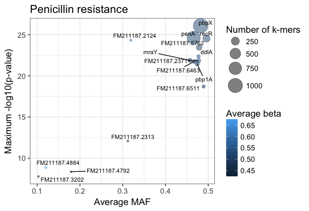
The main hits have high p-values and are common, and in this case are covered by many k-mers. In this case penA (pbp2b) and penX (pbp2x) are the main hits. Other top genes recR and ddl are adjacent to the pbp genes and are in LD with them, creating an artifical association.
The results with large effect sizes (see :ref:`effect-size`) and relatively low p-values also have low MAF, and are probably false positives. This can be seen better by changing the axes:
