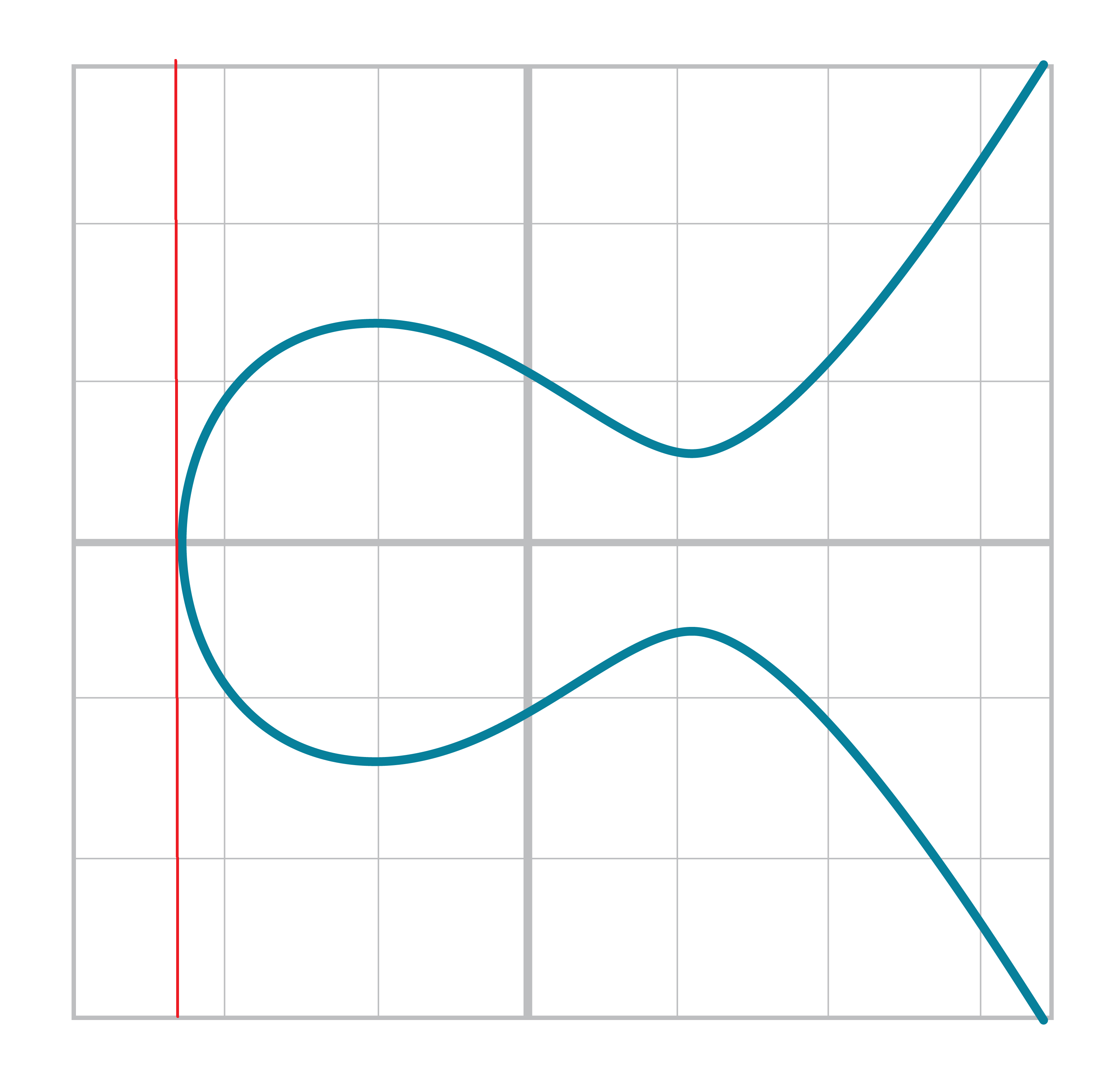
In this chapter we’re going to learn about Elliptic Curves. In the next chapter, we will combine Elliptic Curves with Finite Fields to make Elliptic Curve Cryptography.
As in the previous chapter, elliptic curves can look intimidating if you haven’t seen them before. Also as in the previous chapter, the actual math isn’t very difficult. Most of Elliptic Curves could have been taught to you around the second year of High School. In this chapter, we’ll get to what these curves are and what we can do with them.
Elliptic Curves are really just like many equations you’ve been seeing since around 8th grade. They have y on one side and x on the other in some form. They specifically have a form like this:
y2=x3+ax+b
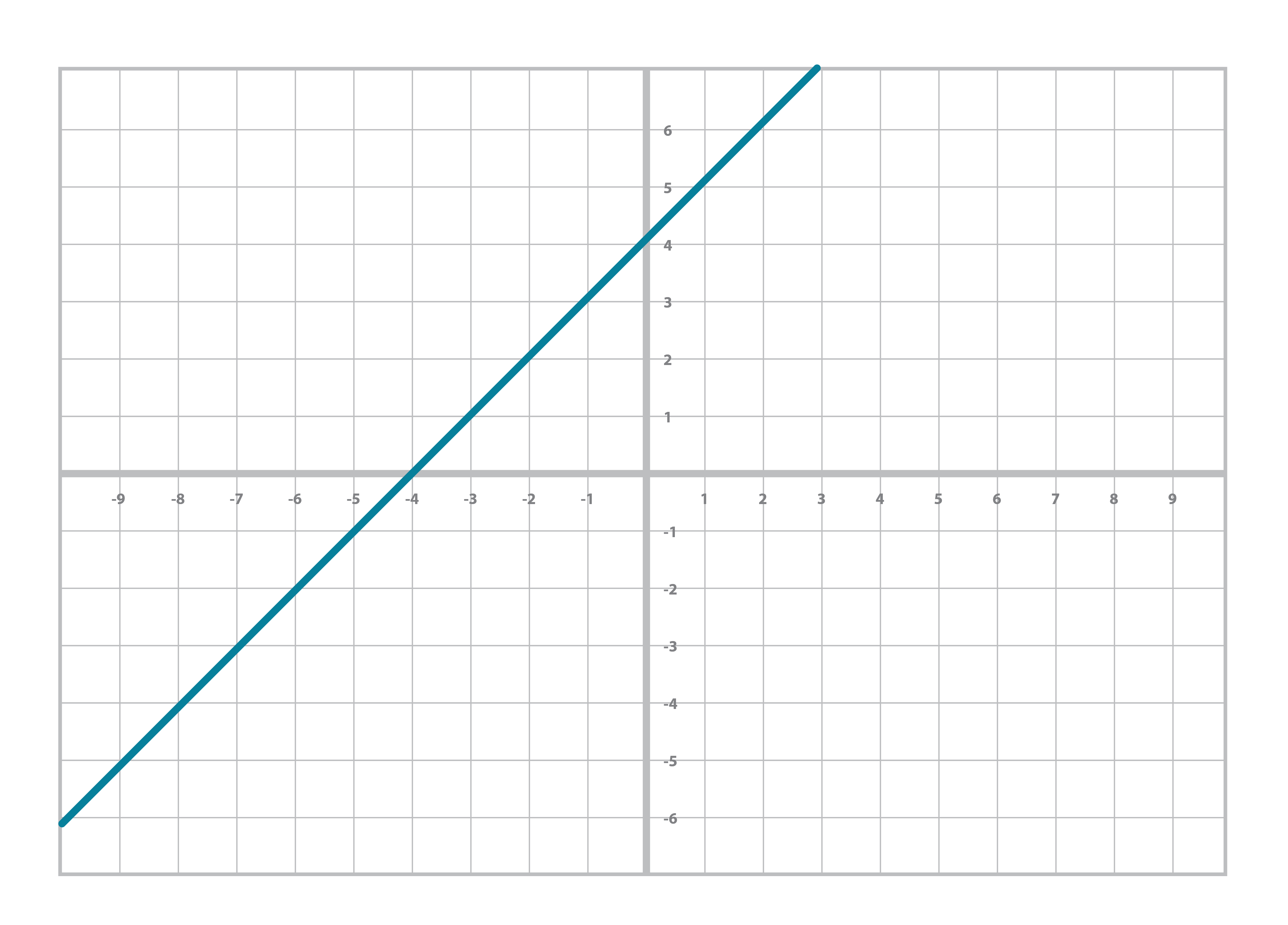
This is probably somewhat familiar as you’ve worked with other equations that look similar. For example, you probably learned the linear equation back in pre-algebra:
y = mx + b
You may even remember that m here has the name slope and b, y-intercept. You can also graph linear equations like this:
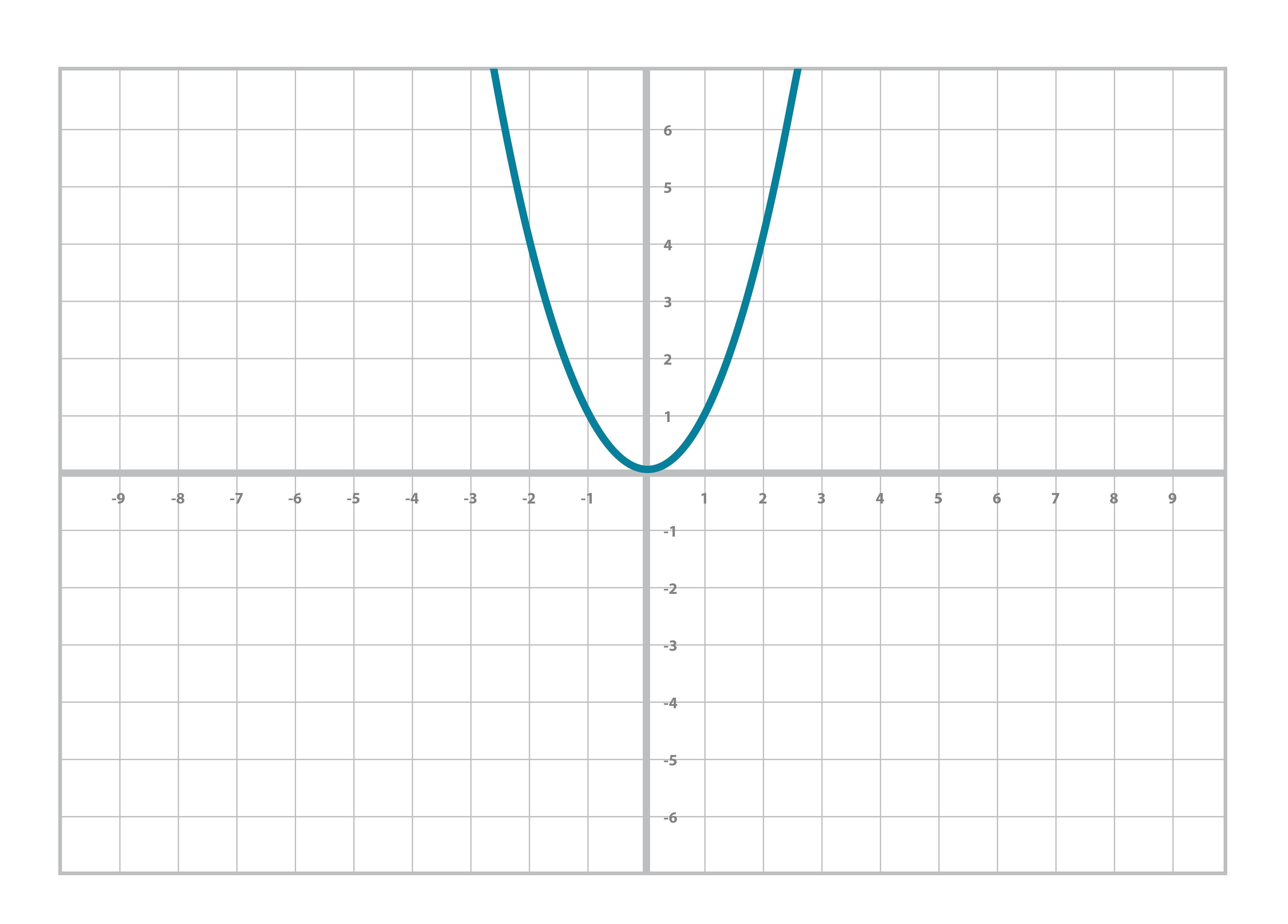
Similarly, you’re probably familiar with the quadratic equation and its graph:
y = ax2+bx+c
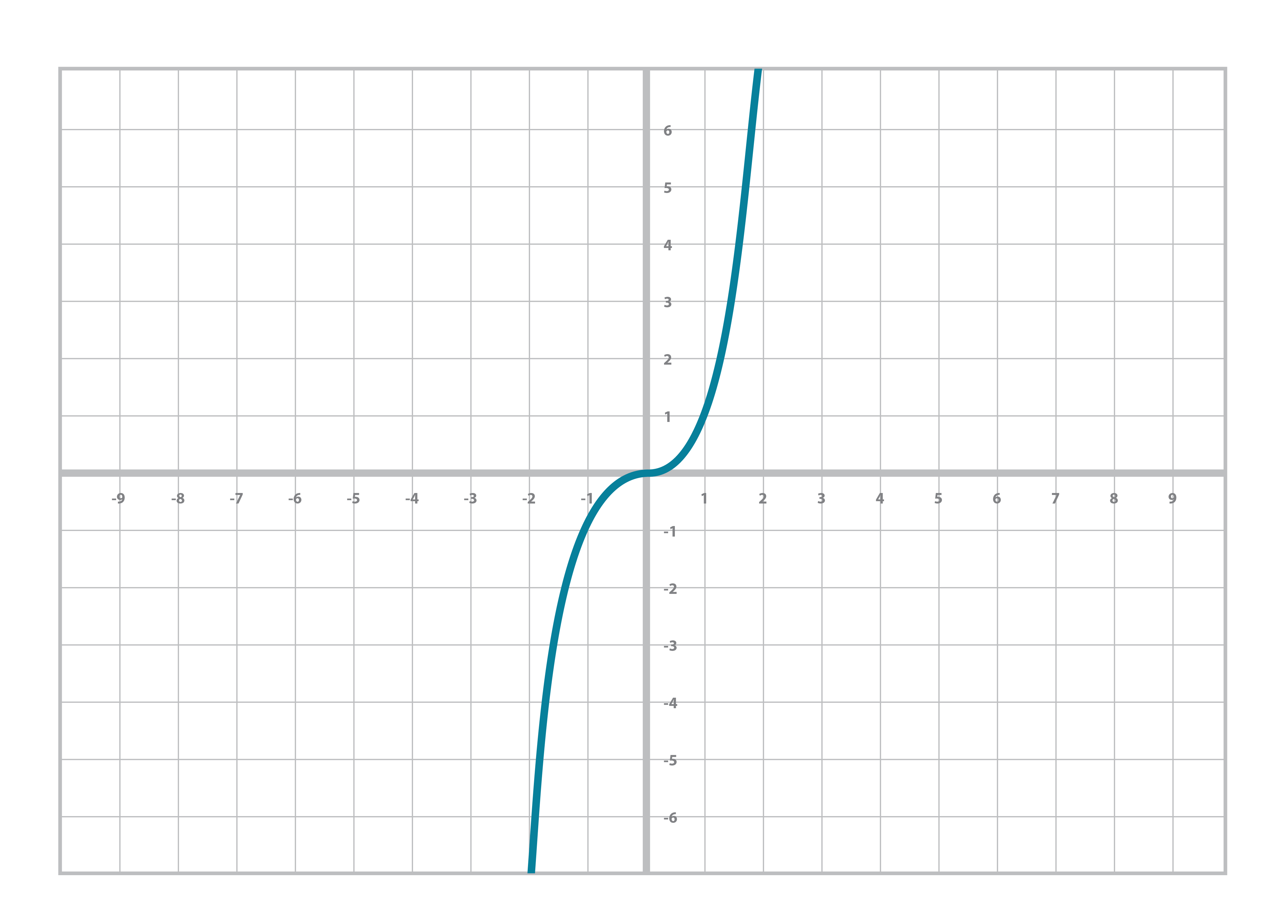
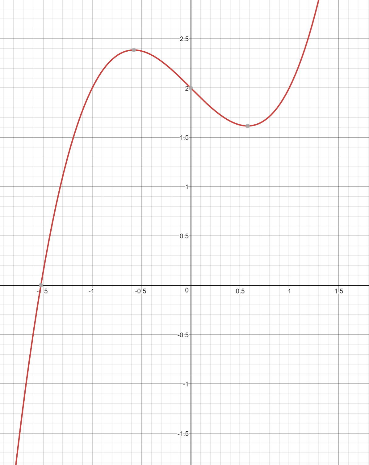
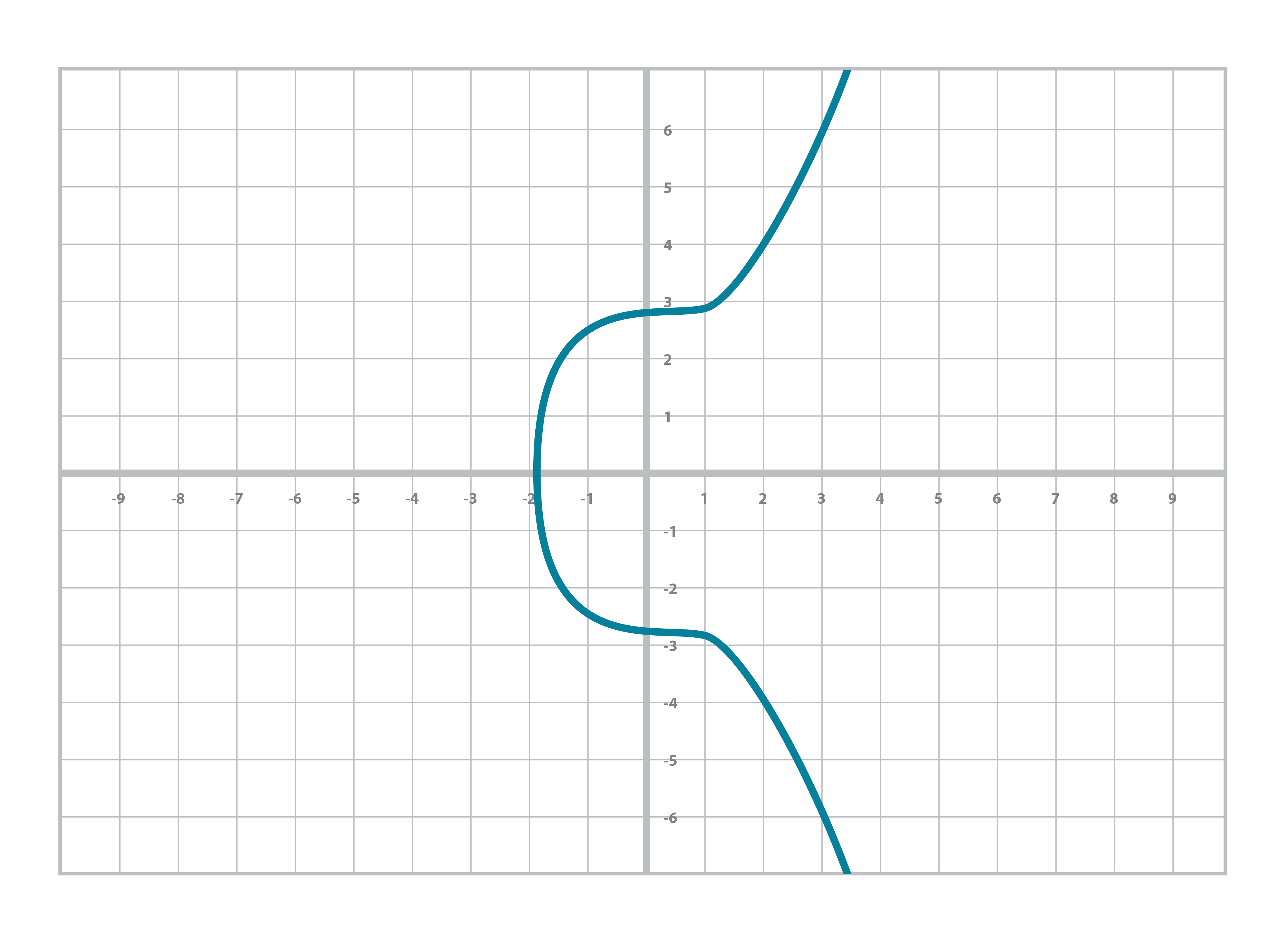
And sometime in high school, you did even higher orders on x, something called the cubic equation and its graph:
y = ax3+bx2+cx+d
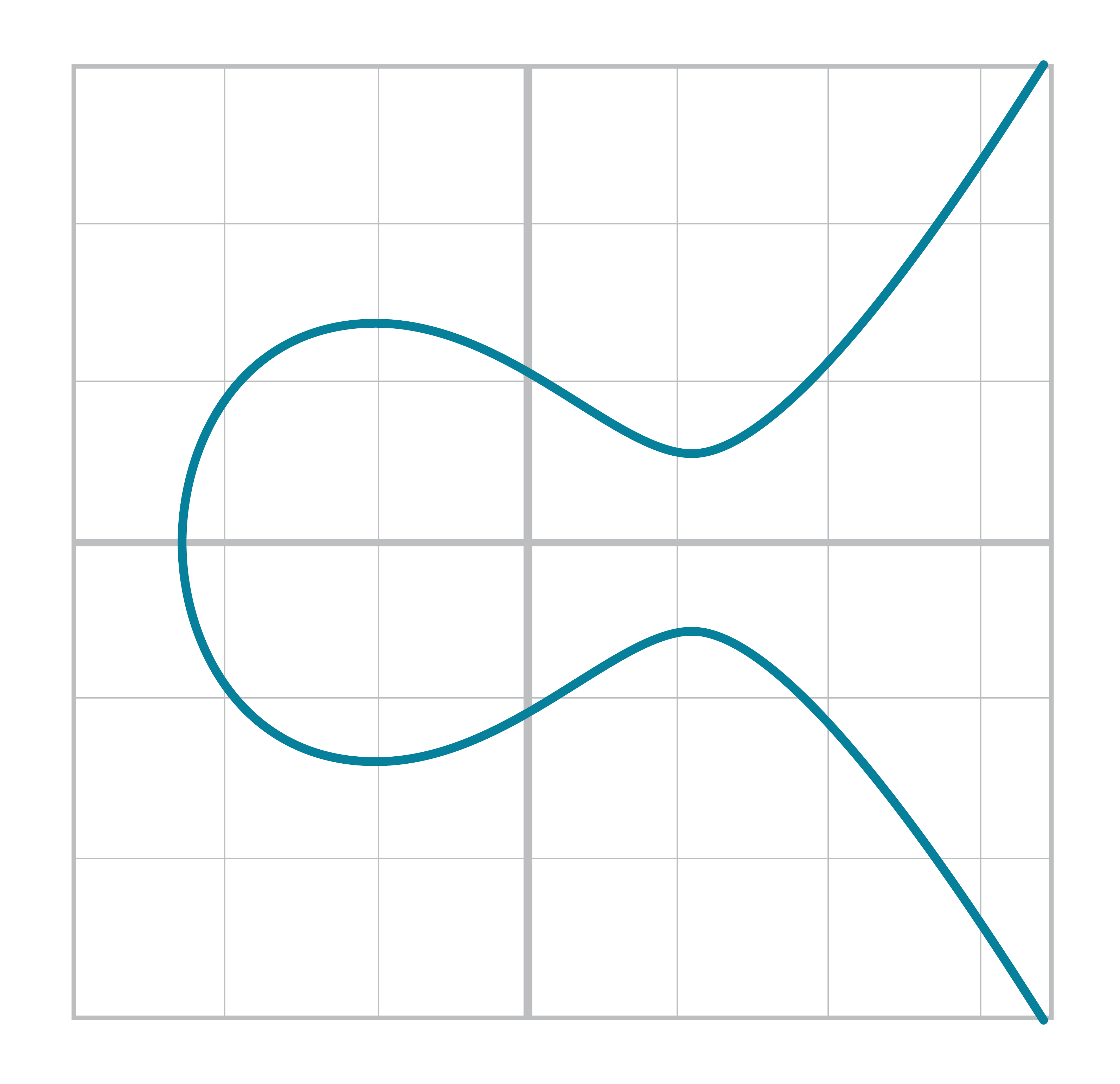
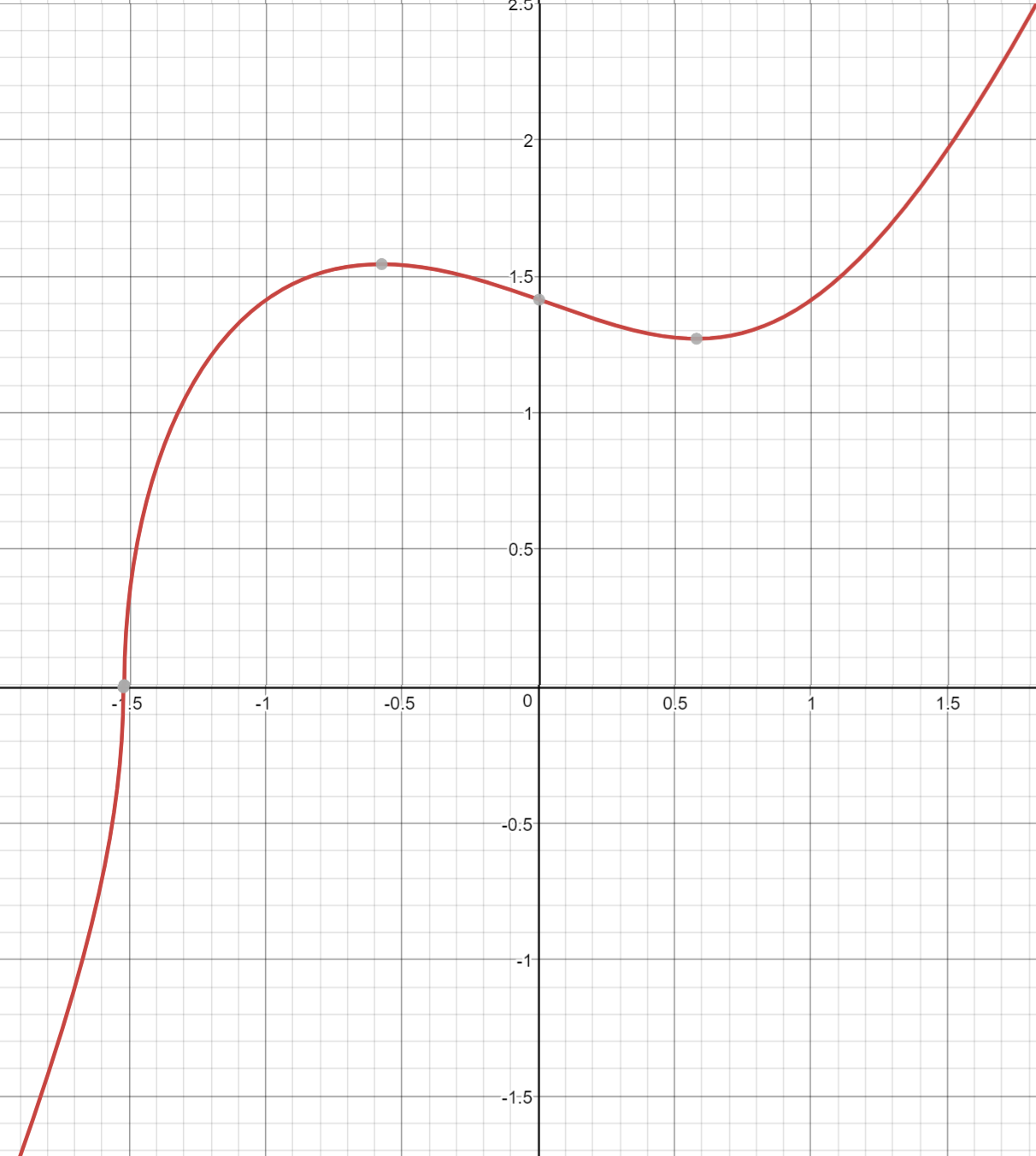
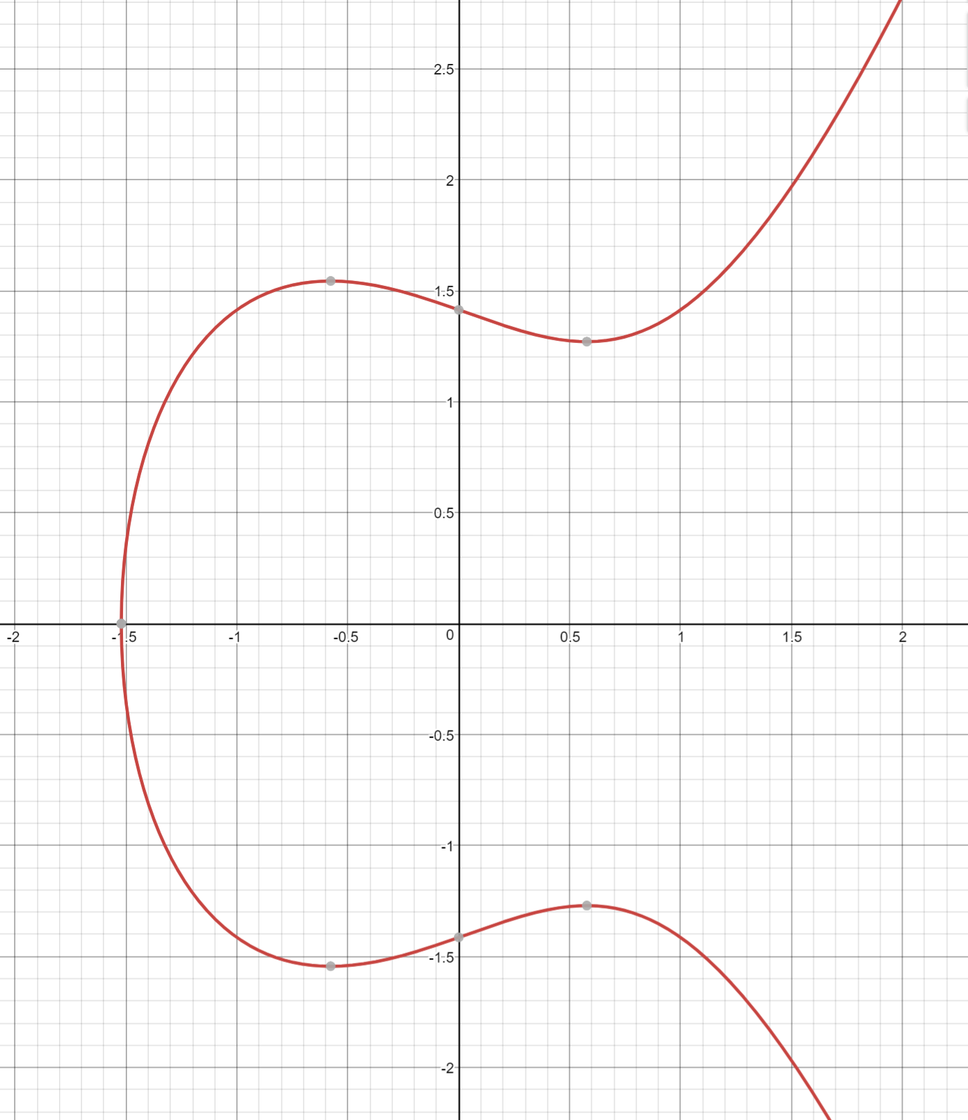
An elliptic curve isn’t all that different. The only real difference between the elliptic curve and the cubic curve above is the y2 term on the right side. This has the effect of making the graph symmetric over the x-axis like so:
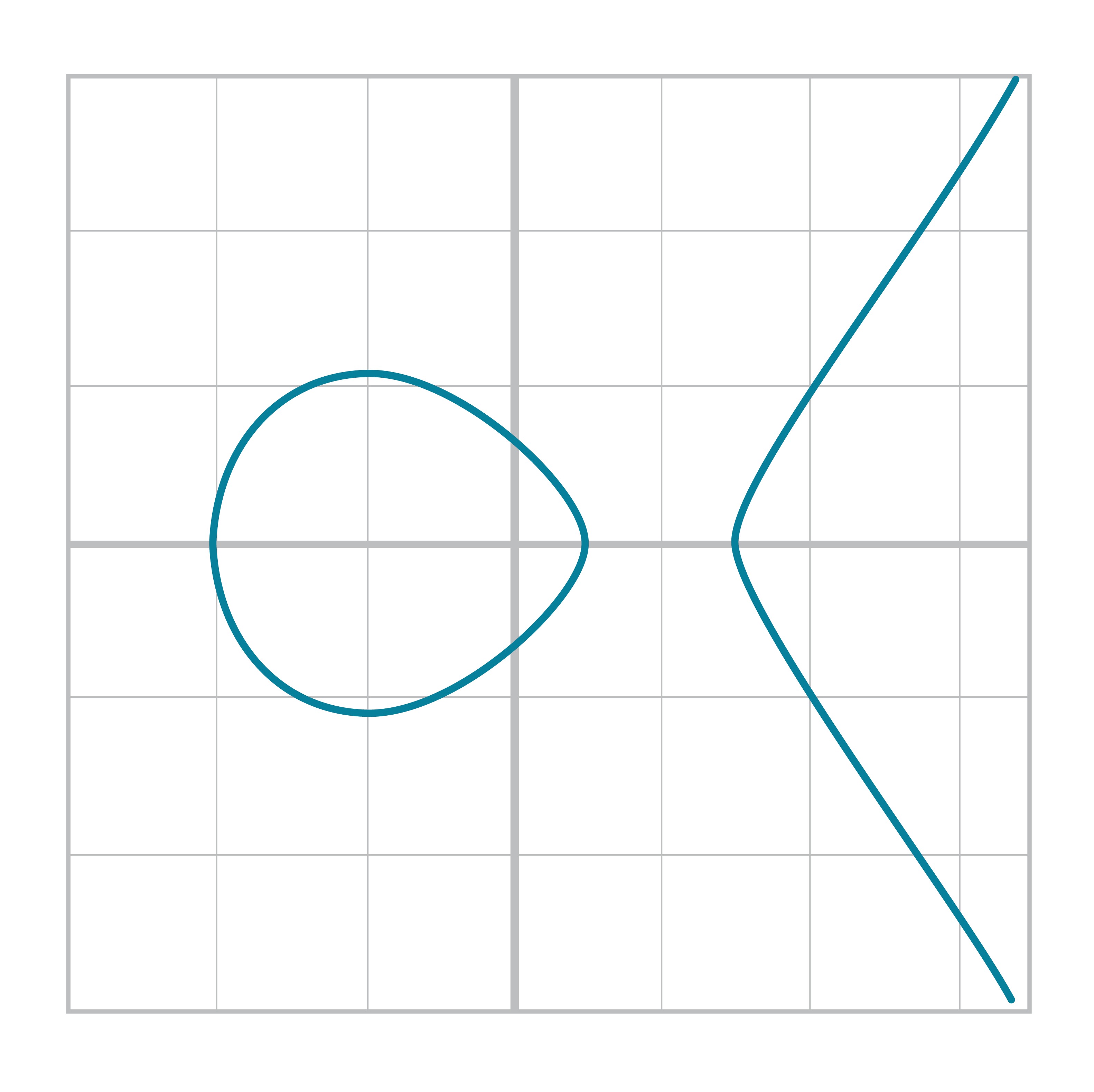
You may also have noticed that the elliptic curve is less steep than the cubic curve. Again, this is because of the y2 term on the right. At times, the curve may even be disjoint like this:
If it helps, an elliptic curve is more or less made by taking a cubic equation graph, taking only the part above the x-axis, flattening it out and then mirroring the top half on the bottom half of the x-axis.
Specifically, the elliptic curve used in Bitcoin is called secp256k1 and it uses this particular equation:
y2=x3+7
The canonical form is y2=x3+ax+b so you can also think of the curve as being a=0, b=7. The curve looks like this:
For a variety of reasons which will be clear later, we are not interested in the curve itself, but specific points on the curve. For example, in the curve y2=x3+5x+7, we are interested in the coordinate (-1,1). We are thus going to define the class Point to be the actual point on a specific curve. The curve has a specifc form, y2=x3+ax+b so we can define the curve with just the two numbers a and b.
class Point:

    def __init__(self, x, y, a, b):
        self.a = a
        self.b = b
        self.x = x
        self.y = y
        if self.y**2 != self.x**3+self.a*self.x + self.b: # (1)
	    raise ValueError('Point ({},{}) is not on the curve'.format(x,y))

    def __eq__(self, other): # (2)
return self.a == other.a and self.b == other.b and self.x == other.x and self.y == other.y-
We check here that the point is actually on the curve.
-
Points are equal iff they are on the same curve and have the same coordinates
This allows us to do something like this:
>>> from ecc import Point
>>> p1 = Point(-1, -1, 5, 7)
>>> p2 = Point(-1, -2, 5, 7)
Traceback (most recent call last):
  File "<stdin>", line 1, in <module>
  File "ecc.py", line 143, in __init__
    raise ValueError('({}, {}) is not on the curve'.format(self.x, self.y))
ValueError: (-1, -2) is not on the curve
We want the __init__ method to throw an error when the point is actually not on the curve.
Determine which of these points are on the curve y2=x3+5x+7:
(2,4), (-1,-1), (18,77), (5,7)
The main reason that Elliptic Curves are useful is because of something called Point Addition. Point Addition is where we can do an operation on two of the points on the curve and get a third point. It’s called addition because it has a lot of the intuitions we associate with what we call "addition". For example, Point Addition is commutative. That is, adding point A to point B is the same as adding point B to point A.
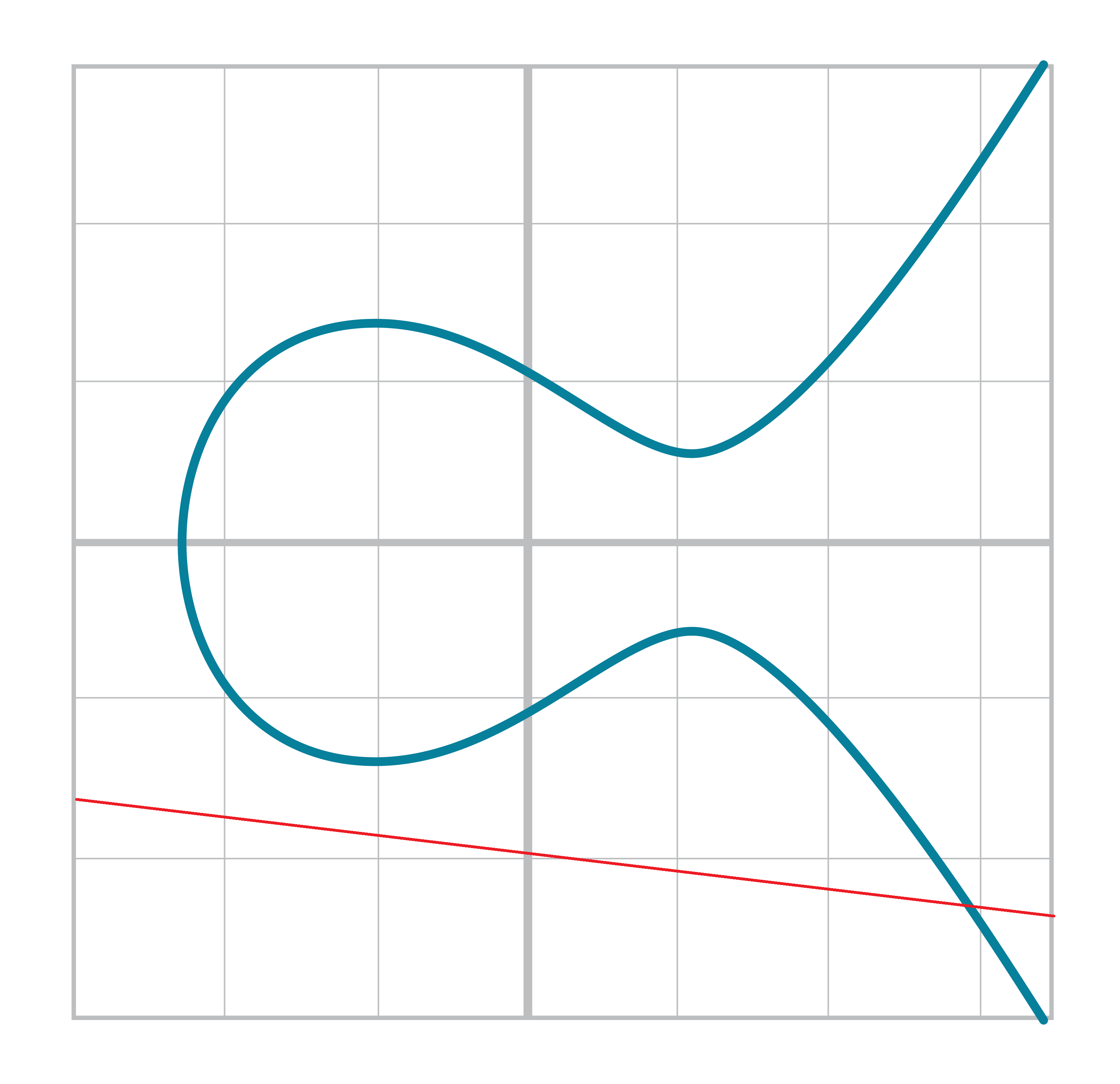
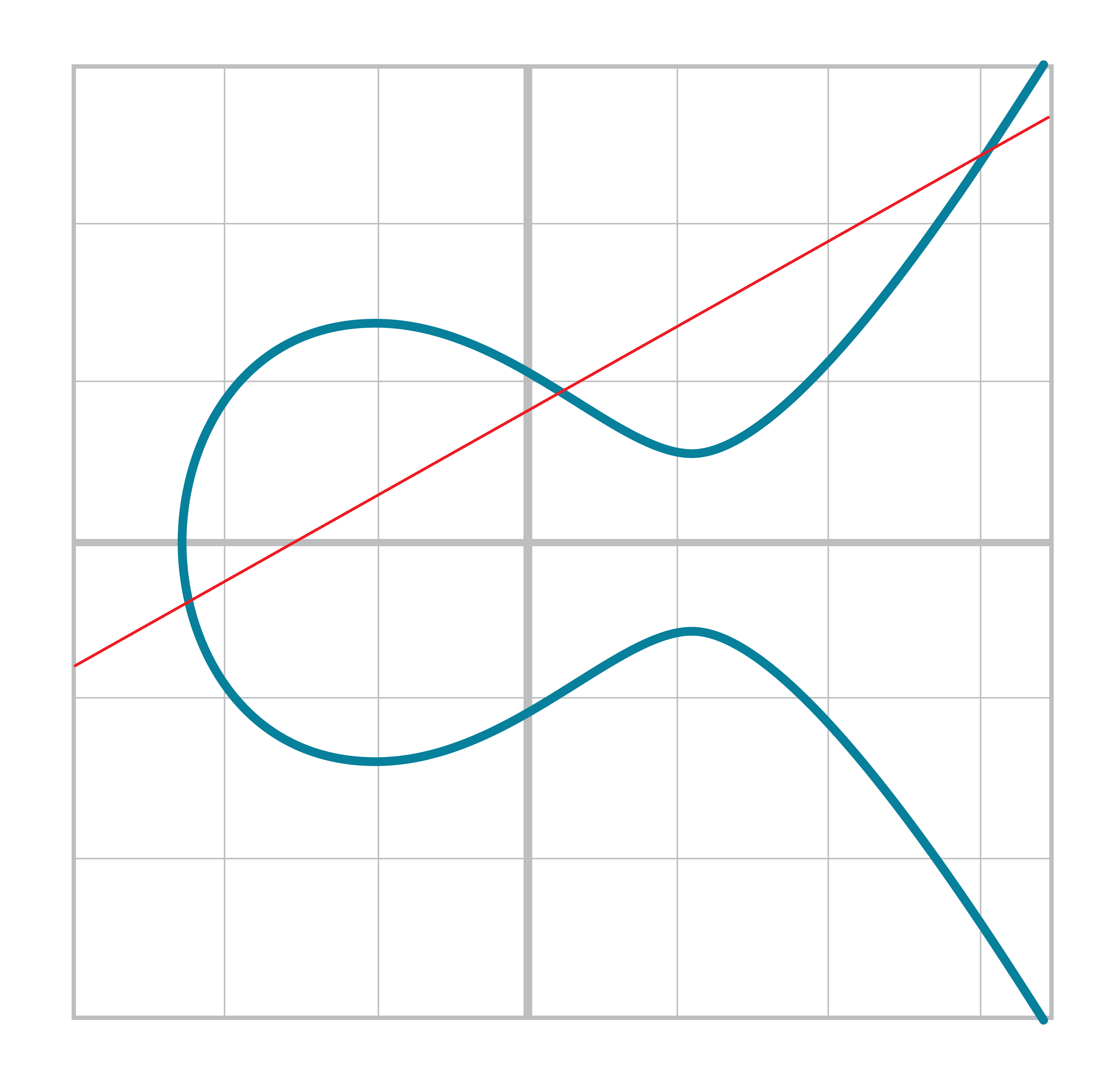
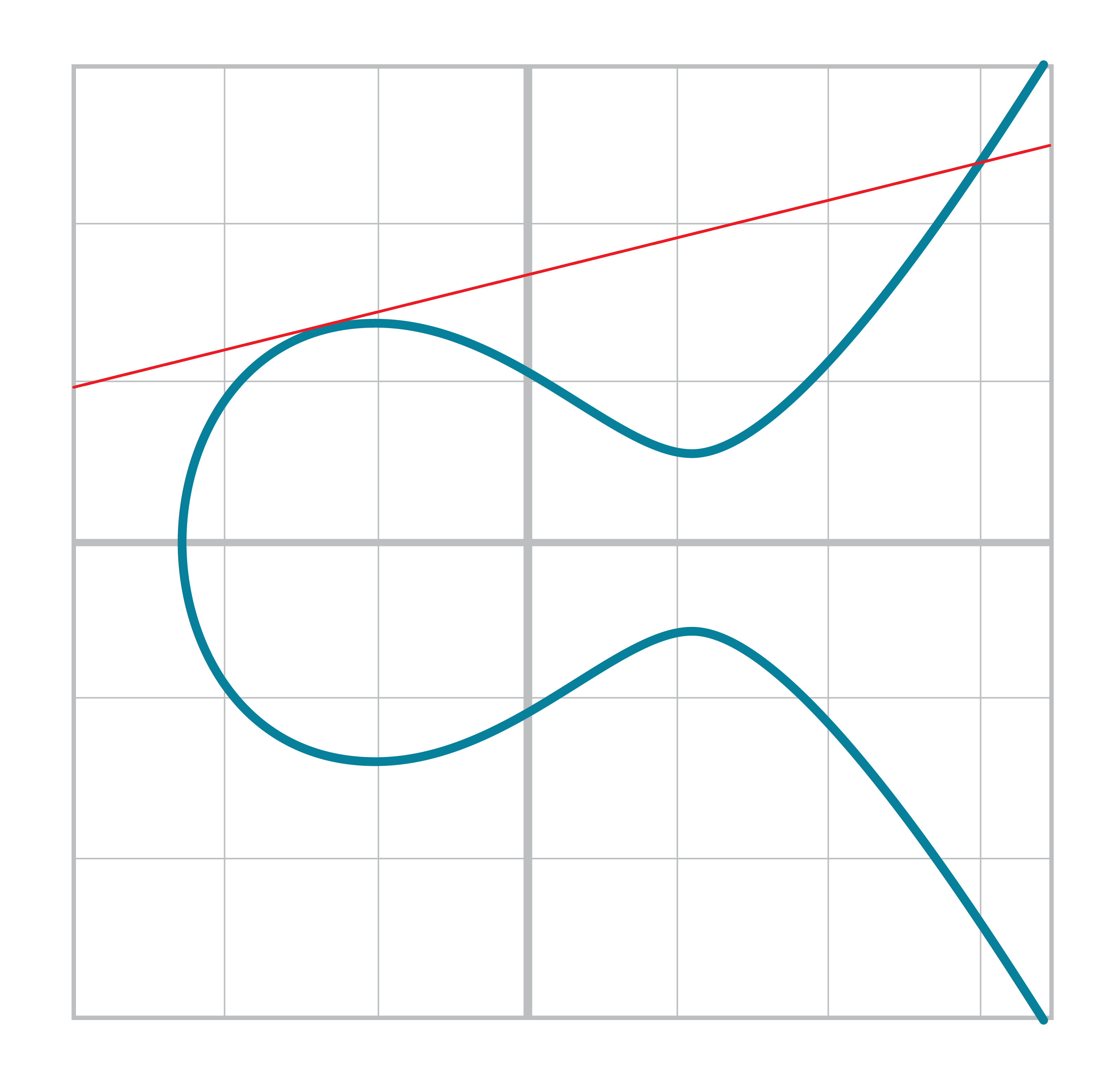
The way we define Point Addition is as follows. It turns out that for every elliptic curve a line, except for a couple of special cases, will intersect at either 1 or 3 points.
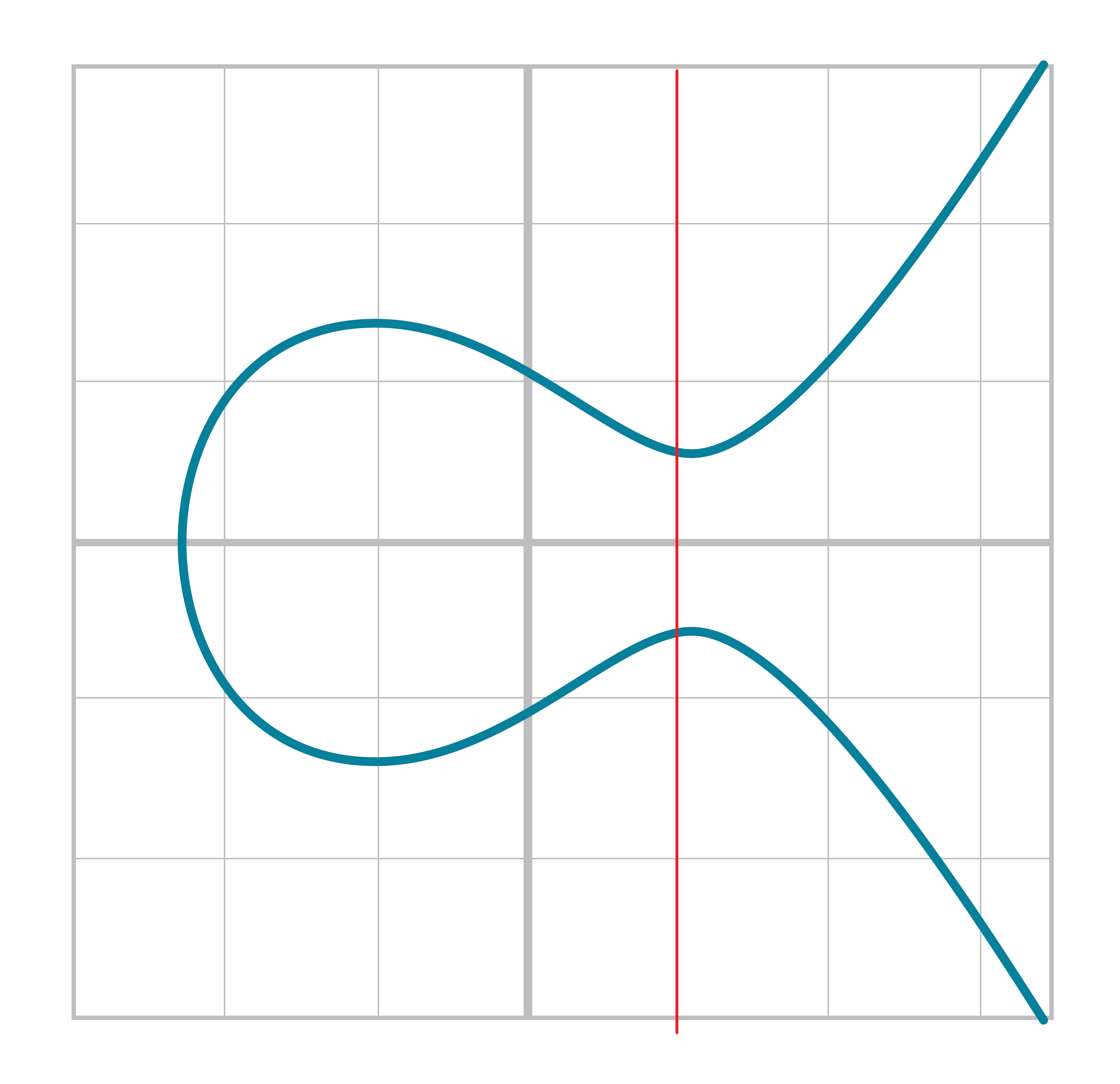
The two exceptions are when a line is tangent to the curve and when a line is exactly vertical.
We will come back to these two cases later.
What’s interesting is that we can define point addition using the fact that lines intersect one or three times with the Elliptic Curve. Two points define a line, so since that line intersects must intersect one more time. That third point reflected over the x-axis is the resulting Point Addition.
Like Field Addition, we are defining Point Addition. In our case, Point Addition is defined this way:
For any two points P1=(x1,y1) and P2=(x2,y2), we get P1+P2 by:
-
Find the point intersecting the elliptic curve a third time by drawing a line through P1 and P2
-
Reflect the resulting point over the x-axis
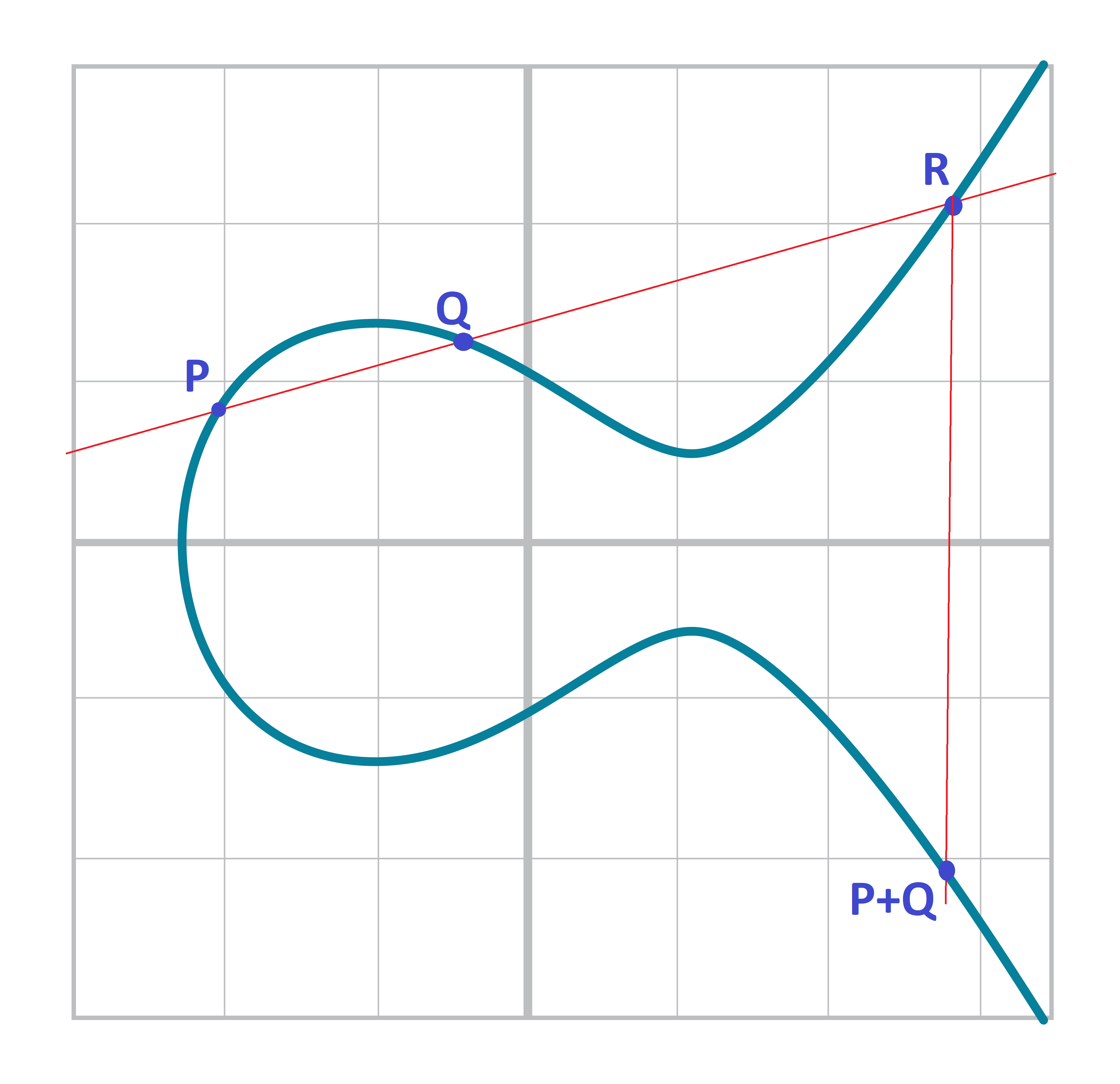
Visually, it looks something like this:
We first draw a line through the two points we’re adding (P and Q). The third intersection point is R. We then reflect that point over the x-axis, which puts us at the P+Q point in Figure 2-14.
One of the properties that we are going to use is that point addition is not easily predictable. We can calculate point addition easily enough with a formula, but intuitively, the result of point addition can be almost anywhere given two points on the curve. Going back to Figure 2-14, P+Q is to the right of both points, P+R would be somewhere between P and R on the x-axis, and Q+R would be to the left of both points. In mathematics parlance, point addition is non-linear.
"Addition" in the name Point Addition satisfies certain properties that we think of as addition, such as:
-
Identity
-
Commutativity
-
Associativity
-
Invertibiltiy
Identity here means that there’s a zero. That is, there exists some point (I) which when added to a point (P) results in P. We’ll call this point the point at infinity (reasons for this will become clear in a bit). That is:
I + P = P
This is also related to invertibility. For some point P, there’s some other point -P which results in the Identity point. That is:
P + (-P) = I
Visually, these are points opposite each other in the elliptic curve.
This is why we call this point the point at infinity. We have one extra point in the elliptic curve which makes the vertical line intersect a third time.
Commutativity means that P+Q=Q+P. This is obvious since the line going through P and Q will intersect the curve a third time in the same place no matter what order.
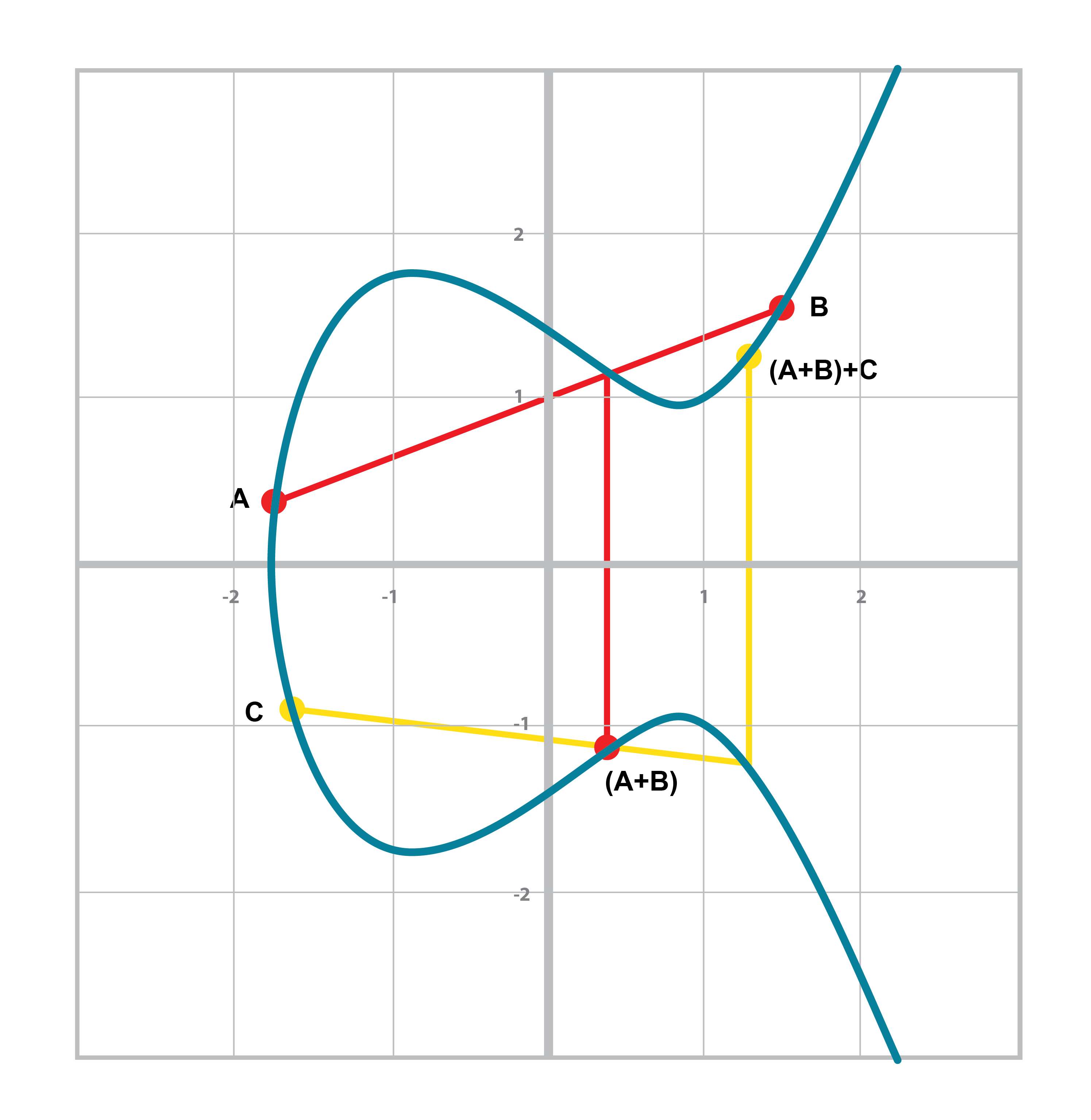
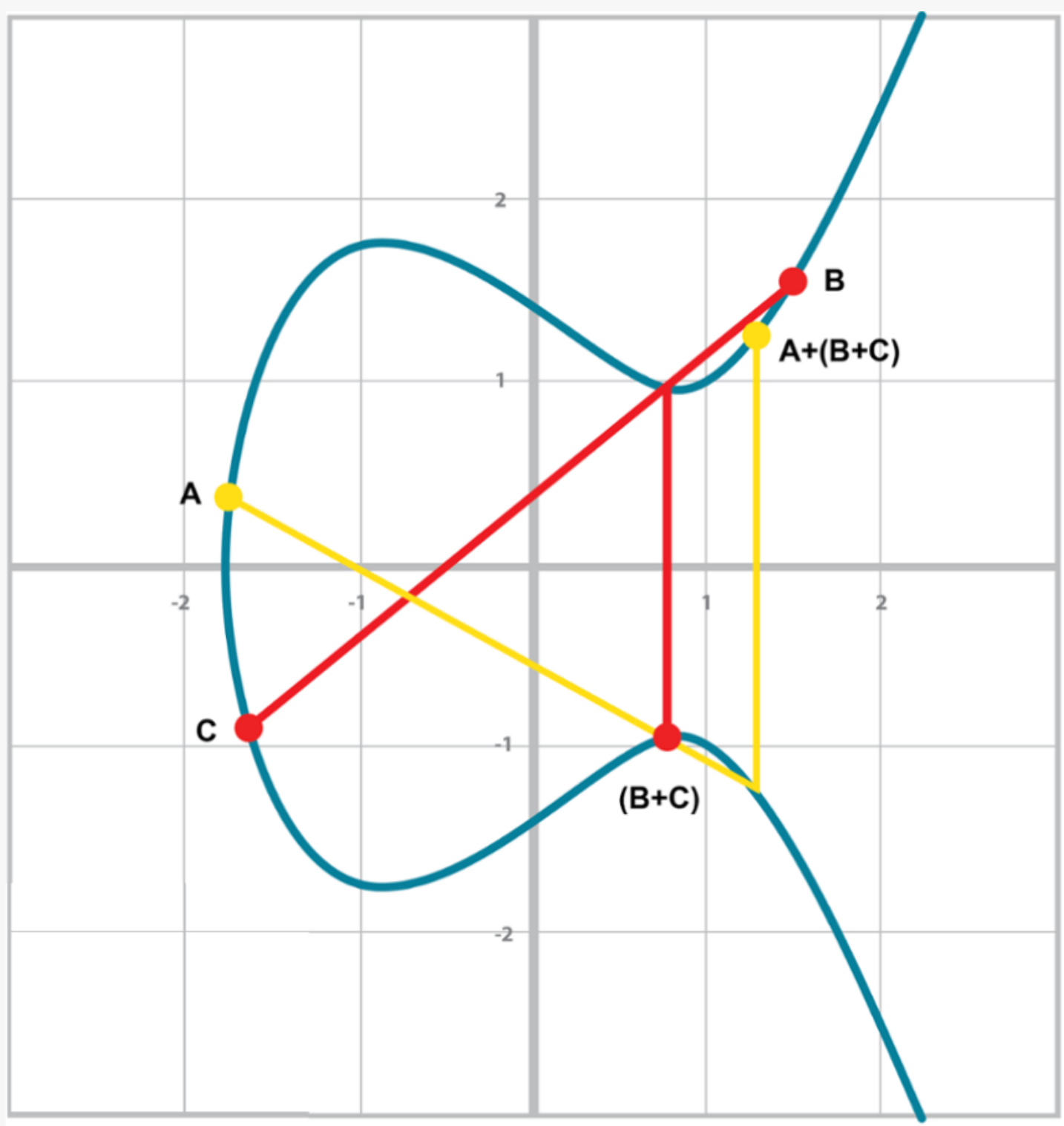
Associativity means that (P+Q) + R = P + (Q+R). This isn’t obvious and is the reason for flipping over the x-axis.
You can see that in both cases, the final point is exactly the same. While this doesn’t prove the associativity of Point addition, the visual should at least give you the intuition that this is true.
To actually do the Point Addition, we’re going to split it up into 3 steps:
-
Where the points are in a vertical line or using the Identity.
-
Where the points are not in a vertical line, but are different.
-
Where the two points are the same.
We first handle the identity, or the point at infinity. Since we don’t have the infinity numbers in Python, we’ll use the None value instead. What we want is something like this:
>>> from ecc import Point
>>> p1 = Point(-1, -1, 5, 7)
>>> p2 = Point(-1, 1, 5, 7)
>>> inf = Point(None, None, 5, 7)
>>> p1 + inf
Point(-1, -1)
>>> inf + p2
Point(-1, 1)
>>> p1 + p2
Point(infinity)
In order to make this work, we have to do two things:
First, we have to adjust the __init__ method slightly so it doesn’t check that the curve equation is satisfied. Second, we have to overload the addition operator or __add__ as we did with the FieldElement class.
class Point:

    def __init__(self, x, y, a, b):
        self.a = a
        self.b = b
        self.x = x
        self.y = y
	if self.x is None and self.y is None:  # (1)
	    return
        if self.y**2 != self.x**3 + self.a*self.x + self.b:
	    raise ValueError('Point ({},{}) is not on the curve'.format(x,y))
    ...

    def __add__(self, other): # (2)
        if self.a != other.a or self.b != other.b:
            raise TypeError('Points {}, {} are not on the same curve'.format(self, other))

    	if self.x is None: # (3)
	    return other
	if other.x is None: # (4)
return self-
x-coordinate and y-coordinate being
Noneis how we signify the point at infinity. Note that the next if statement will fail if we don’t return here. -
We overload the
+operator here -
self.xbeingNonemeans thatselfis the point at infinity, or the additive identity. Thus, we returnother -
self.xbeingNonemeans thatotheris the point at infinity, or the additive identity. Thus, we returnself
Now that we’ve covered the vertical line, we’re now proceeding to when the points are different. As the points are not vertical, the points must have different x-coordinates. When we have points where the x’s differ, we can add using a fairly simple formula. To help with intuition, it helps first to find the slope created by the two points. You can figure this out using a formula from pre-algebra:
P1=(x1,y1), P2=(x2,y2), P3=(x3,y3)
P1+P2=P3
s=(y2-y1)/(x2-x1)
This is the slope and we can figure out where the x3 intersection is. Once we know that, we can calculate y3. P3 can thus be derived using this formula:
x3=s2-x1-x2
y3=s(x1-x3)-y1
Remember that y3 is the reflection over the x-axis.
Supposing:
P1=(x1,y1), P2=(x2,y2), P3=(x3,y3)
P1 + P2 = P3
We want to know what P3 is.
Let’s start with the fact that the line that goes through P1 and P2 looks like this:
s=(y2-y1)/(x2-x1)
y=s(x-x1)+y1
The second formula here is the equation of the line that intersects at both P1 and P2. Now using this formula and plugging it into the elliptic curve equation, we get:
y2=x3+ax+b
y2=(s(x-x1)+y1)2=x3+ax+b
Gathering all the terms, we have this polynomial equation:
x3-s2x2+(a+2s2x1-2sy1)x+b-(sx1-y1)2=0
We also know that x1, x2 and x3 are solutions to this equation, thus:
(x-x1)(x-x2)(x-x3)=0
x3-(x1+x2+x3)x2 +(x1x2+x1x3+x2x3)x-x1x2x3=0
From above, we know that:
x3-s2x2+(a+2s2x1-2sy1)x+b-(sx1-y1)2=0
There’s a result from called the Theorem on the Equality of Polynomials, which states that the coefficients have to equal each other if the roots are the same. The first one that’s interesting is the coefficient in front of x2:
s2=x1+x2+x3
We can use this to derive the formula for x3:
x3=s2-x1-x2
We can plug this in to the formula for the line above:
y=s(x-x1)+y1
But we have to reflect over the x-axis, so this has to be negated:
y3=-(s(x-x1)+y1)=s(x1-x3)-y1
That’s how we arrive at this formula.
We now have to actually code this into our library. That means we have to adjust the __add__ method to handle the case where x1≠x2. We have the formulas:
s=(y2-y1)/(x2-x1)
x3=s2-x1-x2
y3=s(x1-x3)-y1
Now we have to return an instance of the class Point that corresponds to this.
When the x coordinates are the same and the y coordinate is different, we have the situation where the points are opposite each other over the x-axis. We know that this means:
P1=-P2 or P1+P2=I
We’ve already handled this above.
What happens when P1=P2? Visually, we have to calculate the line that’s tangent to the curve at P1 and find the point at which the line intersects the curve. The situation looks like this as we saw before:
Once again, we’ll have to find the slope of the tangent point.
P1=(x1,y1), P3=(x3,y3)
P1+P1=P3
s=(3x12+a)/(2y1)
The rest of the formula goes through as before, except x1=x2, so we can combine them:
x3=s2-2x1
y3=s(x1-x3)-y1
We can derive the slope of the tangent line using some slightly more advanced math: calculus. We know that the slope at a given point is
dy/dx
To get this, we need to take the derivative of both sides of the elliptic curve equation:
y2=x3+ax+b
Taking the derivative we get:
2y dy=(3x2+a) dx
Solving for dy/dx, we get:
dy/dx=(3x2+a)/(2y)
That’s how we arrive at the slope formula. The rest of the results from the point addition formula derivation hold.
Once again, we have to adjust the __add__ method to account for this particular case. We have the formulas, we now have to implement them.
s=(3x12+a)/(2y1)
x3=s2-2x1
y3=s(x1-x3)-y1
There is one more exception and this involves the case where the tangent line is vertical:
This can only happen if P1=P2 and the y-coordinate is 0, in which case the slope calculation will end up with a 0 in the denominator.
We can handle this using a special case:
class Point:
    zero = 0 # (1)
    ...
    def __add__(self, other):
    	...
	if self == other and self.y == self.zero: # (2)
return self.__class__(None, None, self.a, self.b) # (3)-
For reasons which will become clear in the next chapter, we need to define zero specific to the class.
-
If the two points are equal and the y coordinate is zero, we return the point at infinity.
-
This is how we create a point at infinity
