Motion Planning in the Frenet frame

Overview

The Frenet Transform is a tool used in motion planning to decouple lateral and longitudinal control as described in this paper. Open source C++ and Python implementations of the paper are available here and here. The approach samples multiple polynomial trajectories in Frenet coordinates i.e. $s$ and $d$ by varying the terminal condition constraints. This allows for fast parallelized sampling. The trajectories are evaluated with respect to a cost function, and filtered with allowable velocity, acceleration and curvature limits. The trajectory with the lowest cost is then chosen.

Approach

Instead of planning polynomial trajectories in the Frenet coordinate space, an alternative MPC based approach is tested.

MPC System Model

A simple point mass model is used as the MPC model to generate trajectories in $s$ and $d$. The system states are $\mathbf x=[s, \dot s, d, \dot d]$ and the inputs are $\mathbf u = [\ddot s, \ddot d]$. The discrete system propogation model used is:

$s_{t+1} = s_{t} + \dot s_t * \Delta t + \frac{1}{2}\ddot s_t *\Delta t^2$
$d_{t+1} = d_{t} + \dot d_t * \Delta t + \frac{1}{2}\ddot d_t *\Delta t^2$

Cost Function

The cost function used consists of three terms:

1. Deviation cost (penalizing $d$): = $k_d * d^2$
2. Progress cost (incentivizing progress $s$ along path): $-k_s * s^2$
3. Desired velocity cost: $k_{v} * (\dot s - \dot s_{des}$) where $\dot s_{des}$ is the desired progress rate

Here, the scaling factors are tunable parameters which affect the planner performance.

Constraints

Constraints are imposed on progress velocity, as well as input changes as in a standard MPC formulation. Obstacle constraints are formulated as non linear distance constraints of the form. $(s - s_{obs})^2 + (d - d_{obs})^2 > r$ where r is the obstacle clearance distance in the Frenet frame.

Implementation

In the interest of time, the approach is implemented in Python using the do_mpc toolbox for optimal control along with the ma97 IPOPT solver. The approach may also be transferred to C++ using a symbolic framework like casadi. Dependencies:

1. do_mpc
2. ipopt

Re-planning loop

The method produces a sequence of optimal inputs and predicted trajectories in the Frenet coordinate space. The trajectories in Frenet Frame are converted to the Cartesian Frame, where acceleration and curvature filters can be applied on the resulting trajectory. The MPC approach is applied in a receding horizon fashion, where replanning is done after applying the first control input from the optimal sequence of control inputs. A simulated version of this is demonstrated, where it is assumed that the robot reaches the next state of the trajectory at every planning iteration. This can be achieved in the real world by using any standard trajectory tracker.

---

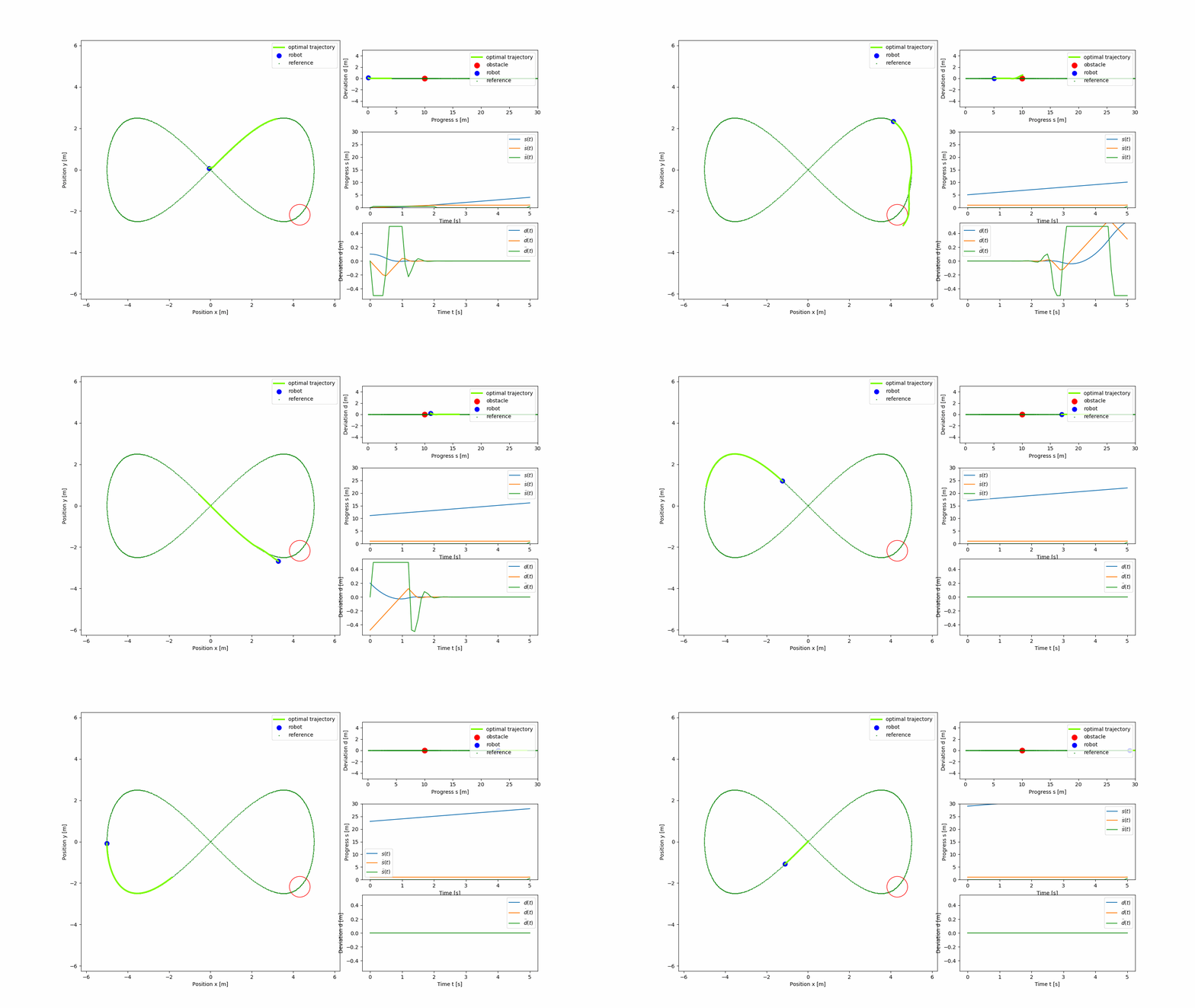
Performance of the planner can be seen in the GIFs below. The figire eight trajectory in Cartesian frame is parameterized as

• $x = a * sin(t)$
• $y = a * cos(t) sin(t)$

These expressions are used when computing the franet transforms.

The light green trajectory is the predicted optimal trajectory from the MPC, and the reference trajectory is shown in green. The states of the MPC over the horizon interval are also shown.

Planning without obstacles

The GIF shows tracking performance without obstacles. The planenr converges to the reference path and maintains zero deviation.

Planning with obstacles

The GIF shows obstacle avoidance behaviour after which the planner continues to track the figure eight trajectory.