Welcome to the lab Instruction!
Instructor Led :
- AWS account - if you don't have one, please ask your instructor for the login detail.
- Source RDS (Postgres) details - Your instructor should provide the database information. Otherwise, follow the instruction in PreLab-instructor and set it up yourself.
Self-Paced : If you want to run pre-requisite steps by yourself
- AWS account - if you don't have one, Sign-up for free AWS account . All sevices in this lab are not covered under free tier, so it may incur some minor cost.
- EC2 Key pair - Follow user guide to create EC2 key pair . You need key pair to deploy cloud formation template in next step. optionally you can login into EC2 with key-pair and interact with RDS database directly using command line.
- To create source RDS database for dataset ingestion - Open the CloudFormation launch template link in a new tab. It will load a CloudFormation Dashboard and start the creation process for your lab environment, which deploys:
    - A source RDS database environment along with Required networking and IAM role setup.
    - Hydrate the source database environment with event tickets sales data
Click the Deploy to AWS icons below to stand up the RDS dataset infrastructure.
| Region | Launch Template |
|---|---|
| N.Virginia (us-east-1) |  |
These labs are designed to be completed in sequence, and the full set of instructions are documented below. Read and follow along to complete the labs. Our lab instructor will give you a high-level overview of the labs and help answer any questions. Don't worry if you get stuck, we provide hints along the way.
Ensure your region is US East (N. Virginia)
- Workshop Setup: Create working environment on AWS
- Lab 1: Hydrateing the data lake via DMS
- Lab 2: Transforming in the data lake with Glue
- Lab 3: Consuming the data lake with Athena & QuickSight
- Lab 4: Machine learning in the data lake
- Lab 5: Modernize Data Warehouse with Amazon Redshift Spectrum
- Cleanup Put everything away nicely
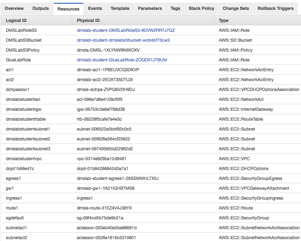
- Open the CloudFormation launch template link in a new tab. It will load a CloudFormation Dashboard and start the creation process for your lab environment, which deploys:
    - A required Virtual Private Cloud for the DMS
    - An Amazon S3 bucket for the Data Lake
    - A required S3 bucket policy to restrict the data access by AWS DMS service
    - A Glue Service Role to use in later hands-on lab
Click the Deploy to AWS icons below to stand up the core workshop infrastructure.
| Region | Launch Template |
|---|---|
| N.Virginia (us-east-1) |  |
- The template will automatically take you to the CloudFormation Console and start the stack creation process in N.Virginia region.
Proceed through the wizard to launch the stack. Leave all options at their default values, but make sure to check the box to allow CloudFormation to create IAM roles on your behalf:
See the Events tab for progress on the stack launch that may take up to 5 minutes. You can also see details of any problems here if the launch fails. Proceed to the next step once the stack status advances to "CREATE_COMPLETE".
- Click in the Output tab and take note of value for BucketName, GlueLabRole and DMSLabRoleS3, which you are going to use in future labs.
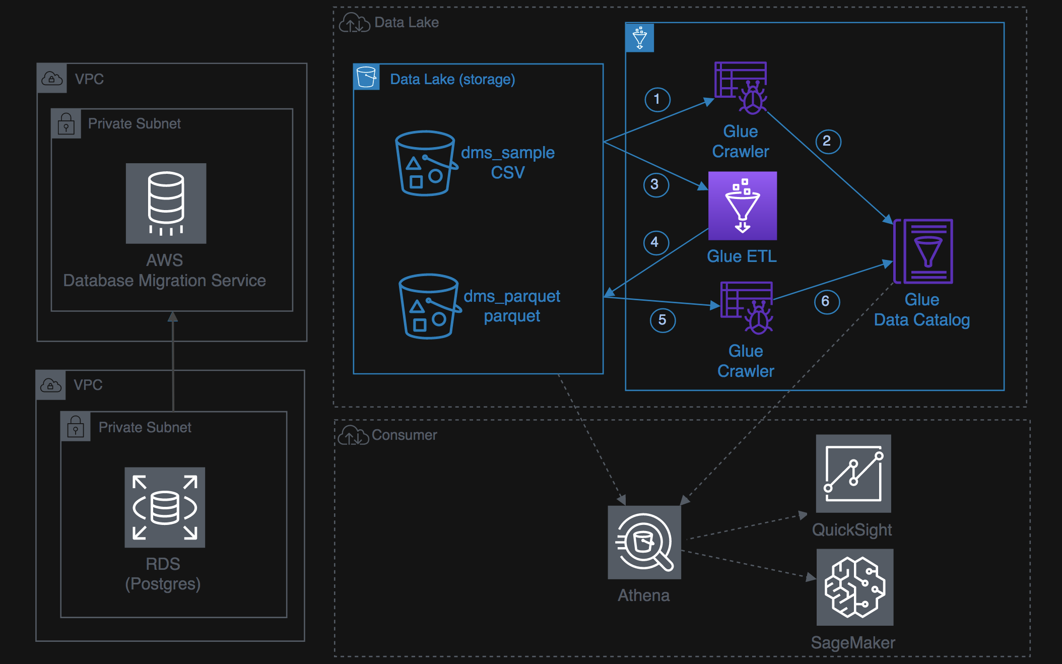
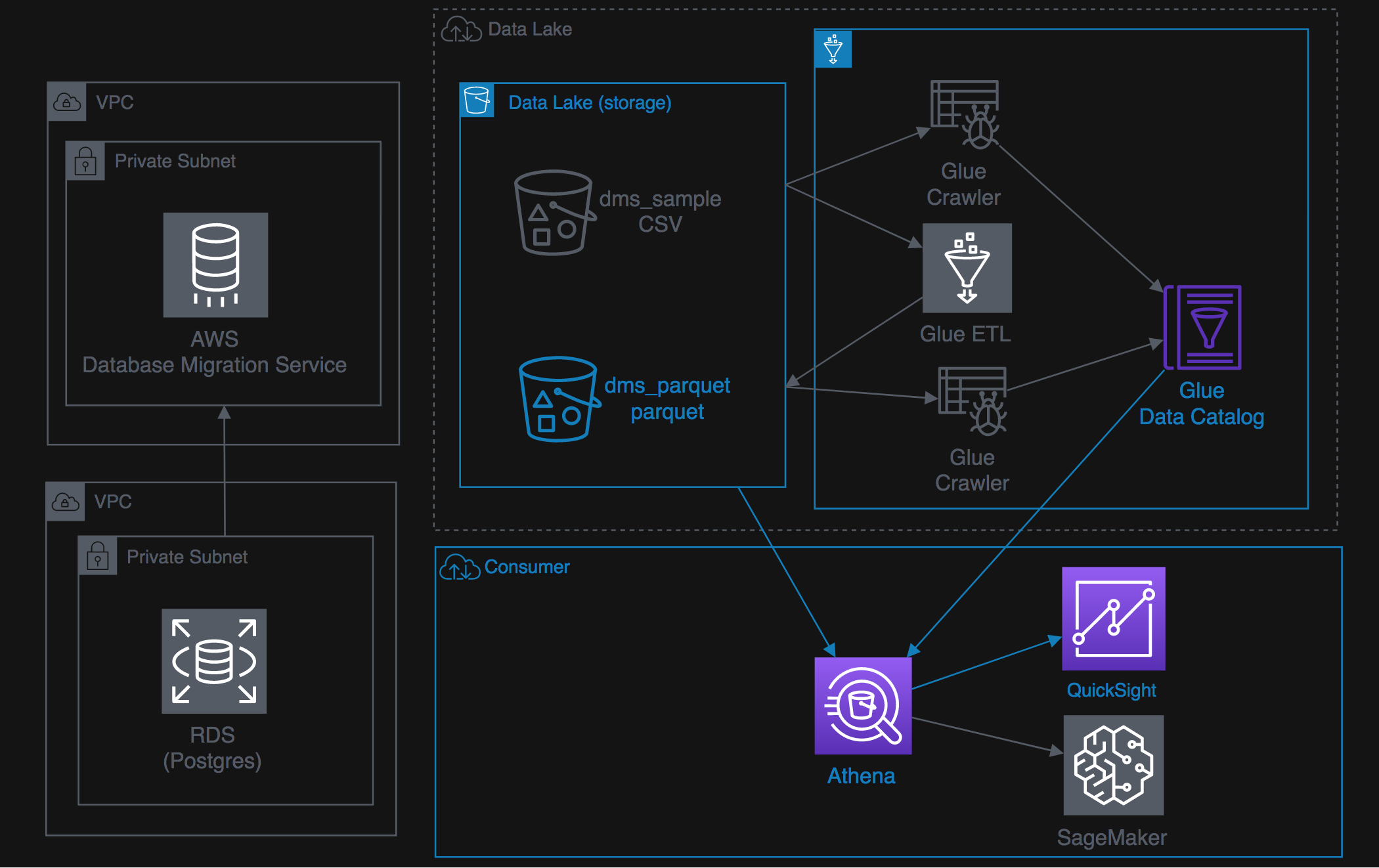
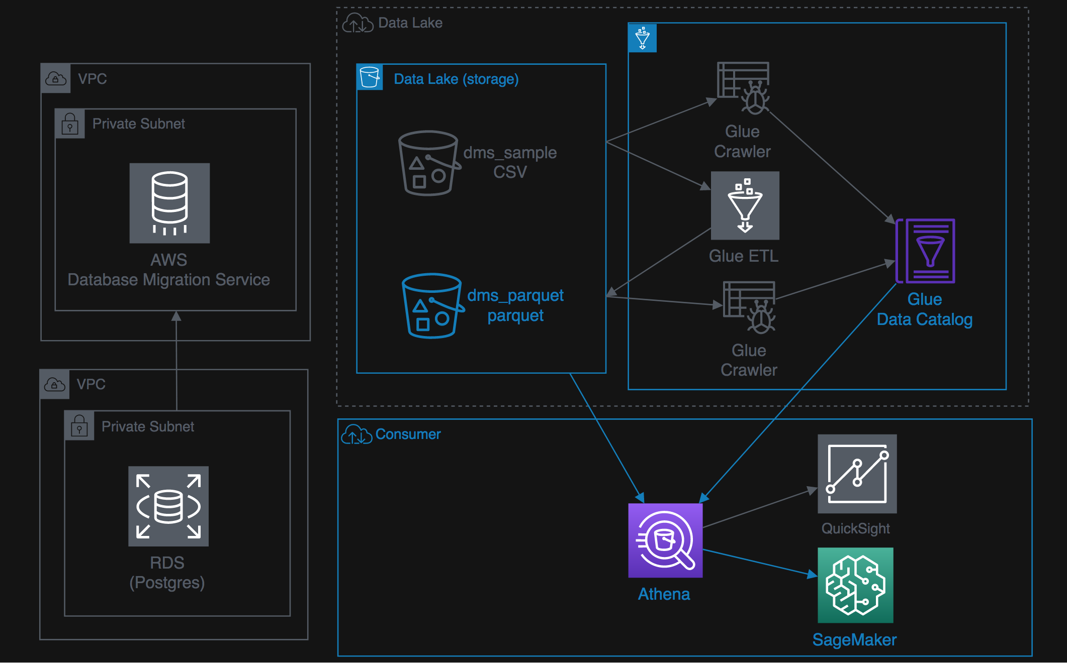
At this point, the data lake workshop environment has been setup, looks like this:
Download the lab1 instruction file
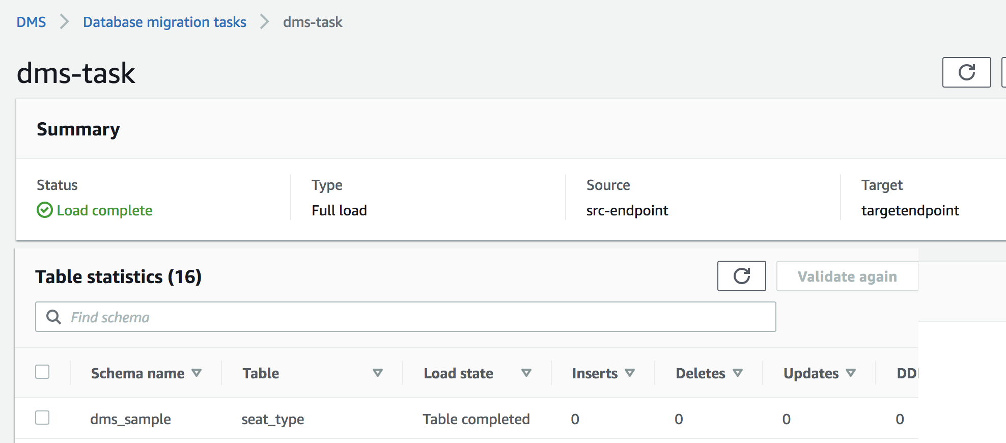
At this point, your DMS task should be finished with 'load Complete' status, and 16 tables are loaded in S3 from RDS by DMS
Download the lab2 instruction file
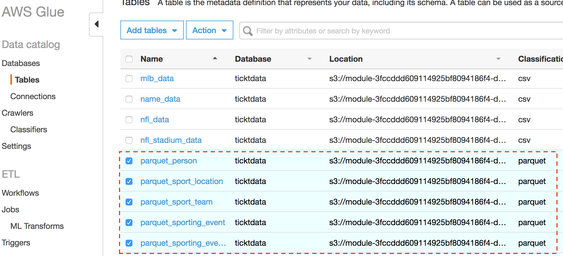
Nice work! You've successfully converted CSV raw data to Parquet, and added parquet tables to the Glue Data Catalog
Download the lab3 instruction file
Sweet! Now you have queried the Data Lake and visualized it in QuickSight. Next, We'll consume the Data Lake via machine learning.
Download the lab4 instruction file
Congratulations, you've successfully built the Data Lake from end to end. If you have time, try the optional steps in the 4 labs above. Otherwise, please remember to follow the steps below in the Workshop Cleanup to make sure all assets created during the workshop are removed so you do not see unexpected charges after today.
In this lab, we show you how to query petabytes of data with Amazon Redshift and exabytes of data in your Amazon S3 data lake, without loading or moving objects. We will also demonstrate how you can leverage views which union data in direct attached storage as well as in your S3 Datalake to create a single source of truth. Finally, we will demonstrate strategies for aging off old data into S3 and maintaining only the most recent data in Amazon Redshift direct attached storage.
- Before You Begin
- What Happened in 2016
- Go Back In Time
- Create a Single Version of Truth
- Plan for the Future
This lab requires a new Redshift cluster in US-WEST-2 (Oregon), use the following link to

And gather the following information from the stack output above:
- [Your-Redshift_Hostname]
- [Your-Redshift_Port]
- [Your-Redshift_Username]
- [Your-Redshift_Password]
- [Your-Redshift_Role_ARN]

In the first part of this lab, we will perform the following activities:
- Load the Green company data for January 2016 into Redshift direct-attached storage (DAS) with COPY.
- Collect supporting/refuting evidence for the impact of the January, 2016 blizzard on taxi usage.
- The CSV data is by month on Amazon S3. Here's a quick screenshot from the S3 console:
https://s3.console.aws.amazon.com/s3/buckets/us-west-2.serverless-analytics/NYC-Pub/green/?region=us-west-2&tab=overview&prefixSearch=green_tripdata_2016
- Here's Sample data from one file which can be previewed directly in the S3 console:
https://s3.console.aws.amazon.com/s3/object/us-west-2.serverless-analytics/NYC-Pub/green/green_tripdata_2013-08.csv?region=us-west-2&tab=select
Login to your query editor, create a schema workshop_das and table workshop_das.green_201601_csv for tables that will reside on the Redshift compute nodes, AKA the Redshift direct-attached storage (DAS) tables.
Hint
CREATE SCHEMA workshop_das;

CREATE TABLE workshop_das.green_201601_csv
(
  vendorid                VARCHAR(4),
  pickup_datetime         TIMESTAMP,
  dropoff_datetime        TIMESTAMP,
  store_and_fwd_flag      VARCHAR(1),
  ratecode                INT,
  pickup_longitude        FLOAT4,
  pickup_latitude         FLOAT4,
  dropoff_longitude       FLOAT4,
  dropoff_latitude        FLOAT4,
  passenger_count         INT,
  trip_distance           FLOAT4,
  fare_amount             FLOAT4,
  extra                   FLOAT4,
  mta_tax                 FLOAT4,
  tip_amount              FLOAT4,
  tolls_amount            FLOAT4,
  ehail_fee               FLOAT4,
  improvement_surcharge   FLOAT4,
  total_amount            FLOAT4,
  payment_type            VARCHAR(4),
  trip_type               VARCHAR(4)
)
DISTSTYLE EVEN
SORTKEY (passenger_count,pickup_datetime);- Build your copy command via Redshift query editor, to copy the data from Amazon S3. This dataset has the number of taxi rides in the month of January 2016.
Hint
COPY workshop_das.green_201601_csv
FROM 's3://us-west-2.serverless-analytics/NYC-Pub/green/green_tripdata_2016-01.csv'
IAM_ROLE '[Your-Redshift_Role_ARN]'
DATEFORMAT 'auto'
IGNOREHEADER 1
DELIMITER ','
IGNOREBLANKLINES
;- Determine how many rows you just loaded.
Hint
select count(1) from workshop_das.green_201601_csv;
--1445285
HINT: The [Your-Redshift_Role_ARN] in the above command should be replaced by the CloudFormation output value at the beginning of the lab.
In this month, there is a date which had the lowest number of taxi rides due to a blizzard. Can you find that date?
SQL-Based Hint
SELECT TO_CHAR(pickup_datetime, 'YYYY-MM-DD'),
COUNT(*)
FROM workshop_das.green_201601_csv
GROUP BY 1
ORDER BY 1;In the next part of this lab, we will perform the following activities:
- Query historical data residing on S3 by create an external DB for Redshift Spectrum.
- Introspect the historical data, perhaps rolling-up the data in novel ways to see trends over time, or other dimensions.
- Enforce reasonable use of the cluster with Redshift Spectrum-specific Query Monitoring Rules (QMR).
- Test the QMR setup by writing an excessive-use query.
Note the partitioning scheme is Year, Month, Type (where Type is a taxi company). Here's a quick Screenshot:
https://s3.console.aws.amazon.com/s3/buckets/serverless-analytics/canonical/NY-Pub/?region=us-west-2&tab=overview
https://s3.console.aws.amazon.com/s3/buckets/serverless-analytics/canonical/NY-Pub/year%253D2016/month%253D1/?region=us-east-1&tab=overview
https://s3.console.aws.amazon.com/s3/buckets/serverless-analytics/canonical/NY-Pub/year%253D2016/month%253D1/type%253Dgreen/?region=us-east-1&tab=overview
Because external tables are stored in a shared Glue Catalog for use within the AWS ecosystem, they can be built and maintained using a few different tools, e.g. Athena, Redshift, and Glue.
-
Use the AWS Glue Crawler to create your external table adb305.ny_pub stored in parquet format under location s3://us-west-2.serverless-analytics/canonical/NY-Pub/.
- Navigate to the Glue Crawler Page. https://console.aws.amazon.com/glue/home?#catalog:tab=crawlers

- Click on Add Crawler, and enter the crawler name NYTaxiCrawler and click Next.

- Select Data stores as the source type and click Next.

- Choose S3 as the data store and the include path of s3://us-west-2.serverless-analytics/canonical/NY-Pub

- Create an IAM Role and enter the name AWSGlueServiceRole-RedshiftImmersion.

- Select Run on demand for the frequency.

- Click on Add database and enter the Database of spectrumdb

- Select all remaining defaults. Once the Crawler has been created, click on Run Crawler.

- Once the Crawler has completed its run, you will see a new table in the Glue Catalog. https://console.aws.amazon.com/glue/home?#catalog:tab=tables

- Click on the ny_pub table, notice the recordCount of 2.87 billion.

- Navigate to the Glue Crawler Page. https://console.aws.amazon.com/glue/home?#catalog:tab=crawlers
-
Now that the table has been cataloged, switch back to your Redshift query editor and create an external schema adb305 pointing to your Glue Catalog Database spectrumdb
Hint
CREATE external SCHEMA adb305
FROM data catalog DATABASE 'spectrumdb'
IAM_ROLE '[Your-Redshift_Role_ARN]'
CREATE external DATABASE if not exists;- Run the query from the previous step using the external table instead of the direct-attached storage (DAS).
Hint
SELECT TO_CHAR(pickup_datetime, 'YYYY-MM-DD'),
COUNT(*)
FROM adb305.ny_pub
WHERE YEAR = 2016 and Month = 01
GROUP BY 1
ORDER BY 1;In Amazon Redshift workload management (WLM), query monitoring rules define metrics-based performance boundaries for WLM queues and specify what action to take when a query goes beyond those boundaries. Setup a Query Monitoring Rule to ensure reasonable use.
https://docs.aws.amazon.com/redshift/latest/dg/cm-c-wlm-query-monitoring-rules.html
Take a look at SVL_QUERY_METRICS_SUMMARY view shows the maximum values of metrics for completed queries. This view is derived from the STL_QUERY_METRICS system table. Use the values in this view as an aid to determine threshold values for defining query monitoring rules.
https://docs.aws.amazon.com/redshift/latest/dg/r_SVL_QUERY_METRICS_SUMMARY.html
Quick Note on QLM: The WLM configuration properties are either dynamic or static. Dynamic properties can be applied to the database without a cluster reboot, but static properties require a cluster reboot for changes to take effect. Additional info here:
https://docs.aws.amazon.com/redshift/latest/mgmt/workload-mgmt-config.html
In the next part of this lab, we will demonstrate how to create a view which has data that is consolidated from S3 via Spectrum and the Redshift direct-attached storage.
Create a view that covers both the January, 2016 Green company DAS table with the historical data residing on S3 to make a single table exclusively for the Green data scientists. Use CTAS to create a table with data from January, 2016 for the Green company. Compare the runtime to populate this with the COPY runtime earlier.
Hint
CREATE TABLE workshop_das.taxi_201601 AS
SELECT * FROM adb305.ny_pub
WHERE year = 2016 AND month = 1 AND type = 'green';
Note: What about column compression/encoding? Remember that on a CTAS, Amazon Redshift automatically assigns compression encoding as follows:
- Columns that are defined as sort keys are assigned RAW compression.
- Columns that are defined as BOOLEAN, REAL, or DOUBLE PRECISION data types are assigned RAW compression.
- All other columns are assigned LZO compression.
https://docs.aws.amazon.com/redshift/latest/dg/r_CTAS_usage_notes.html
ANALYZE COMPRESSION workshop_das.taxi_201601
Here's the output in case you want to use it:
| Column | Encoding | Est_reduction_pct |
|---|---|---|
| vendorid | zstd | 79.46 |
| pickup_datetime | zstd | 33.91 |
| dropoff_datetime | zstd | 34.08 |
| ratecode | zstd | 61.75 |
| passenger_count | zstd | 61.23 |
| trip_distance | zstd | 73.34 |
| fare_amount | bytedict | 85.61 |
| total_amount | zstd | 75.28 |
| payment_type | zstd | 68.76 |
| year | zstd | 91.13 |
| month | zstd | 91.13 |
| type | zstd | 89.23 |
Add to the January, 2016 table with an INSERT/SELECT statement for the other taxi companies.
Hint
INSERT INTO workshop_das.taxi_201601 (
  SELECT *
  FROM adb305.ny_pub
WHERE year = 2016 AND month = 1 AND type != 'green');Now that we've loaded all January, 2016 data, we can remove the partitions from the Spectrum table so there is no overlap between the direct-attached storage (DAS) table and the Spectrum table.
Hint
ALTER TABLE adb305.ny_pub DROP PARTITION(year=2016, month=1, type='fhv');
ALTER TABLE adb305.ny_pub DROP PARTITION(year=2016, month=1, type='green');
ALTER TABLE adb305.ny_pub DROP PARTITION(year=2016, month=1, type='yellow');
Create a view adb305_view_NYTaxiRides from workshop_das.taxi_201601 that allows seamless querying of the DAS and Spectrum data.
Hint
CREATE VIEW adb305_view_NYTaxiRides AS
  SELECT * FROM workshop_das.taxi_201601
  UNION ALL
  SELECT * FROM adb305.ny_pub
WITH NO SCHEMA BINDING;- Note the use of the partition columns in the SELECT and WHERE clauses. Where were those columns in your Spectrum table definition?
- Note the filters being applied either at the partition or file levels in the Spectrum portion of the query (versus the Redshift DAS section).
- If you actually run the query (and not just generate the explain plan), does the runtime surprise you? Why or why not?
EXPLAIN
SELECT year, month, type, COUNT(*)
FROM adb305_view_NYTaxiRides
WHERE year = 2016 AND month IN (1) AND passenger_count = 4
GROUP BY 1,2,3 ORDER BY 1,2,3;
QUERY PLAN
XN Merge  (cost=1000090025653.20..1000090025653.21 rows=2 width=48)
  Merge Key: derived_col1, derived_col2, derived_col3
  ->  XN Network  (cost=1000090025653.20..1000090025653.21 rows=2 width=48)
        Send to leader
        ->  XN Sort  (cost=1000090025653.20..1000090025653.21 rows=2 width=48)
              Sort Key: derived_col1, derived_col2, derived_col3
              ->  XN HashAggregate  (cost=90025653.19..90025653.19 rows=2 width=48)
                    ->  XN Subquery Scan adb305_view_nytaxirides  (cost=25608.12..90025653.17 rows=2 width=48)
                          ->  XN Append  (cost=25608.12..90025653.15 rows=2 width=38)
                                ->  XN Subquery Scan "*SELECT* 1"  (cost=25608.12..25608.13 rows=1 width=18)
                                      ->  XN HashAggregate  (cost=25608.12..25608.12 rows=1 width=18)
                                            ->  XN Seq Scan on t201601_pqt  (cost=0.00..25292.49 rows=31563 width=18)
                                                  <b>Filter: ((passenger_count = 4) AND ("month" = 1) AND ("year" = 2016))</b>
                                ->  XN Subquery Scan "*SELECT* 2"  (cost=90000045.00..90000045.02 rows=1 width=38)
                                      ->  XN HashAggregate  (cost=90000045.00..90000045.01 rows=1 width=38)
                                            ->  XN Partition Loop  (cost=90000000.00..90000035.00 rows=1000 width=38)
                                                  ->  XN Seq Scan PartitionInfo of adb305.nytaxirides  (cost=0.00..15.00 rows=1 width=30)
                                                       <b> Filter: (("month" = 1) AND ("year" = 2016))</b>
                                                  ->  XN S3 Query Scan nytaxirides  (cost=45000000.00..45000010.00 rows=1000 width=8)
                                                        ->  S3 Aggregate  (cost=45000000.00..45000000.00 rows=1000 width=0)
                                                              ->  S3 Seq Scan adb305.nytaxirides location:"s3://us-west-2.serverless-analytics/canonical/NY-Pub" format:PARQUET  (cost=0.00..37500000.00 rows=3000000000 width=0)
                                                                  <b> Filter: (passenger_count = 4)</b>
- Now include Spectrum data by adding a month whose data is in Spectrum
EXPLAIN
SELECT year, month, type, COUNT(*)
FROM adb305_view_NYTaxiRides
WHERE year = 2016 AND month IN (1,2) AND passenger_count = 4
GROUP BY 1,2,3 ORDER BY 1,2,3;
QUERY PLAN
XN Merge  (cost=1000090029268.92..1000090029268.92 rows=2 width=48)
  Merge Key: derived_col1, derived_col2, derived_col3
  ->  XN Network  (cost=1000090029268.92..1000090029268.92 rows=2 width=48)
        Send to leader
        ->  XN Sort  (cost=1000090029268.92..1000090029268.92 rows=2 width=48)
              Sort Key: derived_col1, derived_col2, derived_col3
              ->  XN HashAggregate  (cost=90029268.90..90029268.90 rows=2 width=48)
                    ->  XN Subquery Scan adb305_view_nytaxirides  (cost=29221.33..90029268.88 rows=2 width=48)
                          ->  XN Append  (cost=29221.33..90029268.86 rows=2 width=38)
                                ->  XN Subquery Scan "*SELECT* 1"  (cost=29221.33..29221.34 rows=1 width=18)
                                      ->  XN HashAggregate  (cost=29221.33..29221.33 rows=1 width=18)
                                            ->  XN Seq Scan on t201601_pqt  (cost=0.00..28905.70 rows=31563 width=18)
                                                 <b> Filter: ((passenger_count = 4) AND ("year" = 2016) AND (("month" = 1) OR ("month" = 2))) </b>
                                ->  XN Subquery Scan "*SELECT* 2"  (cost=90000047.50..90000047.52 rows=1 width=38)
                                      ->  XN HashAggregate  (cost=90000047.50..90000047.51 rows=1 width=38)
                                            ->  XN Partition Loop  (cost=90000000.00..90000037.50 rows=1000 width=38)
                                                  ->  XN Seq Scan PartitionInfo of adb305.nytaxirides  (cost=0.00..17.50 rows=1 width=30)
                                                       <b> Filter: (("year" = 2016) AND (("month" = 1) OR ("month" = 2)))</b>
                                                  ->  XN S3 Query Scan nytaxirides  (cost=45000000.00..45000010.00 rows=1000 width=8)
                                                        ->  S3 Aggregate  (cost=45000000.00..45000000.00 rows=1000 width=0)
                                                              ->  S3 Seq Scan adb305.nytaxirides location:"s3://us-west-2.serverless-analytics/canonical/NY-Pub" format:PARQUET  (cost=0.00..37500000.00 rows=3000000000 width=0)
                                                                  <b> Filter: (passenger_count = 4)</b>
EXPLAIN
SELECT passenger_count, COUNT(*)
FROM adb305.ny_pub
WHERE year = 2016 AND month IN (1,2)
GROUP BY 1 ORDER BY 1;
QUERY PLAN
XN Merge  (cost=1000090005026.64..1000090005027.14 rows=200 width=12)
  <b>Merge Key: nytaxirides.derived_col1</b>
  ->  XN Network  (cost=1000090005026.64..1000090005027.14 rows=200 width=12)
        Send to leader
        ->  XN Sort  (cost=1000090005026.64..1000090005027.14 rows=200 width=12)
              <b>Sort Key: nytaxirides.derived_col1</b>
              ->  XN HashAggregate  (cost=90005018.50..90005019.00 rows=200 width=12)
                    ->  XN Partition Loop  (cost=90000000.00..90004018.50 rows=200000 width=12)
                          ->  XN Seq Scan PartitionInfo of adb305.nytaxirides  (cost=0.00..17.50 rows=1 width=0)
                               Filter: (("year" = 2016) AND (("month" = 1) OR ("month" = 2)))
                          ->  XN S3 Query Scan nytaxirides  (cost=45000000.00..45002000.50 rows=200000 width=12)
                                <b> ->  S3 HashAggregate  (cost=45000000.00..45000000.50 rows=200000 width=4)</b>
                                      ->  S3 Seq Scan adb305.nytaxirides location:"s3://us-west-2.serverless-analytics/canonical/NY-Pub" format:PARQUET  (cost=0.00..30000000.00 rows=3000000000 width=4)
EXPLAIN
SELECT type, COUNT(*)
FROM adb305.ny_pub
WHERE year = 2016 AND month IN (1,2)
GROUP BY 1 ORDER BY 1 ;
QUERY PLAN
XN Merge  (cost=1000075000042.52..1000075000042.52 rows=1 width=30)
  <b>Merge Key: nytaxirides."type"</b>
  ->  XN Network  (cost=1000075000042.52..1000075000042.52 rows=1 width=30)
        Send to leader
        ->  XN Sort  (cost=1000075000042.52..1000075000042.52 rows=1 width=30)
              <b>Sort Key: nytaxirides."type"</b>
              ->  XN HashAggregate  (cost=75000042.50..75000042.51 rows=1 width=30)
                    ->  XN Partition Loop  (cost=75000000.00..75000037.50 rows=1000 width=30)
                          ->  XN Seq Scan PartitionInfo of adb305.nytaxirides  (cost=0.00..17.50 rows=1 width=22)
                               Filter: (("year" = 2016) AND (("month" = 1) OR ("month" = 2)))
                          ->  XN S3 Query Scan nytaxirides  (cost=37500000.00..37500010.00 rows=1000 width=8)
                              <b>  ->  S3 Aggregate  (cost=37500000.00..37500000.00 rows=1000 width=0)</b>
                                      ->  S3 Seq Scan adb305.nytaxirides location:"s3://us-west-2.serverless-analytics/canonical/NY-Pub" format:PARQUET  (cost=0.00..30000000.00 rows=3000000000 width=0)
In this final part of this lab, we will compare different strategies for maintaining more recent or HOT data within Redshift direct-attached storage, and keeping older COLD data in S3 by performing the following steps:
-
Allow for trailing 5 quarters reporting by adding the Q4 2015 data to Redshift DAS:
- Anticipating that we’ll want to ”age-off” the oldest quarter on a 3 month basis, architect your DAS table to make this easy to maintain and query.
- Adjust your Redshift Spectrum table to exclude the Q4 2015 data.
-
Develop and execute a plan to move the Q4 2015 data to S3.
- What are the discrete steps to be performed?
- What extra-Redshift functionality must be leveraged?
- Simulating the extra-Redshift steps with the existing Parquet data, age-off the Q4 2015 data from Redshift DAS and perform any needed steps to maintain a single version of the truth.
-
There are several options to accomplish this goal. Anticipating that we’ll want to ”age-off” the oldest quarter on a 3 month basis, architect your DAS table to make this easy to maintain and query. How about something like this?
CREATE OR REPLACE VIEW adb305_view_NYTaxiRides AS
  SELECT * FROM workshop_das.taxi_201504
UNION ALL
  SELECT * FROM workshop_das.taxi_201601
UNION ALL
  SELECT * FROM workshop_das.taxi_201602
UNION ALL
  SELECT * FROM workshop_das.taxi_201603
UNION ALL
  SELECT * FROM workshop_das.taxi_201604
UNION ALL
  SELECT * FROM adb305.ny_pub
WITH NO SCHEMA BINDING;
- Or something like this? Bulk DELETE-s in Redshift are actually quite fast (with one-time single-digit minute time to VACUUM), so this is also a valid configuration as well:
CREATE OR REPLACE VIEW adb305_view_NYTaxiRides AS
   SELECT * FROM workshop_das.taxi_current
UNION ALL
  SELECT * FROM adb305.ny_pub
WITH NO SCHEMA BINDING;
- If needed, the Redshift DAS tables can also be populated from the Parquet data with COPY. Note: This will highlight a data design when we created the Parquet data
COPY with Parquet doesn’t currently include a way to specify the partition columns as sources to populate the target Redshift DAS table. The current expectation is that since there’s no overhead (performance-wise) and little cost in also storing the partition data as actual columns on S3, customers will store the partition column data as well.
- We’re going to show how to work with the scenario where this pattern wasn’t followed. Use the single table option for this example
CREATE TABLE workshop_das.taxi_current
DISTSTYLE EVEN
SORTKEY(year, month, type) AS
SELECT * FROM adb305.ny_pub WHERE 1 = 0;
- And, create a helper table that doesn't include the partition columns from the Redshift Spectrum table.
CREATE TABLE workshop_das.taxi_loader AS
  SELECT vendorid, pickup_datetime, dropoff_datetime, ratecode, passenger_count,
  	trip_distance, fare_amount, total_amount, payment_type
  FROM workshop_das.taxi_current
  WHERE 1 = 0;
- The population could be scripted easily; there are also a few different patterns that could be followed. Below is a script which issues a seperate copy command for each partition where the type=green. Once complete, seperate scripts would need to be used for other type partitions.
COPY workshop_das.taxi_loader FROM 's3://us-west-2.serverless-analytics/canonical/NY-Pub/year=2015/month=10/type=green' IAM_ROLE '[Your-Redshift_Role_ARN]' FORMAT AS PARQUET;
COPY workshop_das.taxi_loader FROM 's3://us-west-2.serverless-analytics/canonical/NY-Pub/year=2015/month=11/type=green' IAM_ROLE '[Your-Redshift_Role_ARN]' FORMAT AS PARQUET;
COPY workshop_das.taxi_loader FROM 's3://us-west-2.serverless-analytics/canonical/NY-Pub/year=2015/month=12/type=green' IAM_ROLE '[Your-Redshift_Role_ARN]' FORMAT AS PARQUET;
COPY workshop_das.taxi_loader FROM 's3://us-west-2.serverless-analytics/canonical/NY-Pub/year=2016/month=1/type=green' IAM_ROLE '[Your-Redshift_Role_ARN]' FORMAT AS PARQUET;
COPY workshop_das.taxi_loader FROM 's3://us-west-2.serverless-analytics/canonical/NY-Pub/year=2016/month=2/type=green' IAM_ROLE '[Your-Redshift_Role_ARN]' FORMAT AS PARQUET;
COPY workshop_das.taxi_loader FROM 's3://us-west-2.serverless-analytics/canonical/NY-Pub/year=2016/month=3/type=green' IAM_ROLE '[Your-Redshift_Role_ARN]' FORMAT AS PARQUET;
COPY workshop_das.taxi_loader FROM 's3://us-west-2.serverless-analytics/canonical/NY-Pub/year=2016/month=4/type=green' IAM_ROLE '[Your-Redshift_Role_ARN]' FORMAT AS PARQUET;
COPY workshop_das.taxi_loader FROM 's3://us-west-2.serverless-analytics/canonical/NY-Pub/year=2016/month=5/type=green' IAM_ROLE '[Your-Redshift_Role_ARN]' FORMAT AS PARQUET;
COPY workshop_das.taxi_loader FROM 's3://us-west-2.serverless-analytics/canonical/NY-Pub/year=2016/month=6/type=green' IAM_ROLE '[Your-Redshift_Role_ARN]' FORMAT AS PARQUET;
COPY workshop_das.taxi_loader FROM 's3://us-west-2.serverless-analytics/canonical/NY-Pub/year=2016/month=7/type=green' IAM_ROLE '[Your-Redshift_Role_ARN]' FORMAT AS PARQUET;
COPY workshop_das.taxi_loader FROM 's3://us-west-2.serverless-analytics/canonical/NY-Pub/year=2016/month=8/type=green' IAM_ROLE '[Your-Redshift_Role_ARN]' FORMAT AS PARQUET;
COPY workshop_das.taxi_loader FROM 's3://us-west-2.serverless-analytics/canonical/NY-Pub/year=2016/month=9/type=green' IAM_ROLE '[Your-Redshift_Role_ARN]' FORMAT AS PARQUET;
COPY workshop_das.taxi_loader FROM 's3://us-west-2.serverless-analytics/canonical/NY-Pub/year=2016/month=10/type=green' IAM_ROLE '[Your-Redshift_Role_ARN]' FORMAT AS PARQUET;
COPY workshop_das.taxi_loader FROM 's3://us-west-2.serverless-analytics/canonical/NY-Pub/year=2016/month=11/type=green' IAM_ROLE '[Your-Redshift_Role_ARN]' FORMAT AS PARQUET;
COPY workshop_das.taxi_loader FROM 's3://us-west-2.serverless-analytics/canonical/NY-Pub/year=2016/month=12/type=green' IAM_ROLE '[Your-Redshift_Role_ARN]' FORMAT AS PARQUET;
INSERT INTO workshop_das.taxi_current
  SELECT *, DATE_PART(year,pickup_datetime), DATE_PART(month,pickup_datetime), 'green'
  FROM workshop_das.taxi_loader;
TRUNCATE workshop_das.taxi_loader;
DROP TABLE IF EXISTS workshop_das.taxi_201601;
CREATE TABLE workshop_das.taxi_201601 AS SELECT * FROM adb305.ny_pub WHERE year = 2016 AND month IN (1,2,3);
CREATE TABLE workshop_das.taxi_201602 AS SELECT * FROM adb305.ny_pub WHERE year = 2016 AND month IN (4,5,6);
CREATE TABLE workshop_das.taxi_201603 AS SELECT * FROM adb305.ny_pub WHERE year = 2016 AND month IN (7,8,9);
CREATE TABLE workshop_das.taxi_201604 AS SELECT * FROM adb305.ny_pub WHERE year = 2016 AND month IN (10,11,12);
Note for the Redshift Editor users: Adjust accordingly based on how many of the partitions you added above.
ALTER TABLE adb305.ny_pub DROP PARTITION(year=2015, month=10, type='fhv');
ALTER TABLE adb305.ny_pub DROP PARTITION(year=2015, month=10, type='yellow');
ALTER TABLE adb305.ny_pub DROP PARTITION(year=2015, month=10, type='green');
ALTER TABLE adb305.ny_pub DROP PARTITION(year=2015, month=11, type='yellow');
ALTER TABLE adb305.ny_pub DROP PARTITION(year=2015, month=11, type='fhv');
ALTER TABLE adb305.ny_pub DROP PARTITION(year=2015, month=11, type='green');
ALTER TABLE adb305.ny_pub DROP PARTITION(year=2015, month=12, type='yellow');
ALTER TABLE adb305.ny_pub DROP PARTITION(year=2015, month=12, type='fhv');
ALTER TABLE adb305.ny_pub DROP PARTITION(year=2015, month=12, type='green');
ALTER TABLE adb305.ny_pub DROP PARTITION(year=2016, month=1, type='yellow');
ALTER TABLE adb305.ny_pub DROP PARTITION(year=2016, month=1, type='fhv');
ALTER TABLE adb305.ny_pub DROP PARTITION(year=2016, month=1, type='green');
ALTER TABLE adb305.ny_pub DROP PARTITION(year=2016, month=2, type='yellow');
ALTER TABLE adb305.ny_pub DROP PARTITION(year=2016, month=2, type='fhv');
ALTER TABLE adb305.ny_pub DROP PARTITION(year=2016, month=2, type='green');
ALTER TABLE adb305.ny_pub DROP PARTITION(year=2016, month=3, type='yellow');
ALTER TABLE adb305.ny_pub DROP PARTITION(year=2016, month=3, type='fhv');
ALTER TABLE adb305.ny_pub DROP PARTITION(year=2016, month=3, type='green');
ALTER TABLE adb305.ny_pub DROP PARTITION(year=2016, month=4, type='yellow');
ALTER TABLE adb305.ny_pub DROP PARTITION(year=2016, month=4, type='fhv');
ALTER TABLE adb305.ny_pub DROP PARTITION(year=2016, month=4, type='green');
ALTER TABLE adb305.ny_pub DROP PARTITION(year=2016, month=5, type='yellow');
ALTER TABLE adb305.ny_pub DROP PARTITION(year=2016, month=5, type='fhv');
ALTER TABLE adb305.ny_pub DROP PARTITION(year=2016, month=5, type='green');
ALTER TABLE adb305.ny_pub DROP PARTITION(year=2016, month=6, type='yellow');
ALTER TABLE adb305.ny_pub DROP PARTITION(year=2016, month=6, type='fhv');
ALTER TABLE adb305.ny_pub DROP PARTITION(year=2016, month=6, type='green');
ALTER TABLE adb305.ny_pub DROP PARTITION(year=2016, month=7, type='yellow');
ALTER TABLE adb305.ny_pub DROP PARTITION(year=2016, month=7, type='fhv');
ALTER TABLE adb305.ny_pub DROP PARTITION(year=2016, month=7, type='green');
ALTER TABLE adb305.ny_pub DROP PARTITION(year=2016, month=8, type='yellow');
ALTER TABLE adb305.ny_pub DROP PARTITION(year=2016, month=8, type='fhv');
ALTER TABLE adb305.ny_pub DROP PARTITION(year=2016, month=8, type='green');
ALTER TABLE adb305.ny_pub DROP PARTITION(year=2016, month=9, type='yellow');
ALTER TABLE adb305.ny_pub DROP PARTITION(year=2016, month=9, type='fhv');
ALTER TABLE adb305.ny_pub DROP PARTITION(year=2016, month=9, type='green');
ALTER TABLE adb305.ny_pub DROP PARTITION(year=2016, month=10, type='yellow');
ALTER TABLE adb305.ny_pub DROP PARTITION(year=2016, month=10, type='fhv');
ALTER TABLE adb305.ny_pub DROP PARTITION(year=2016, month=10, type='green');
ALTER TABLE adb305.ny_pub DROP PARTITION(year=2016, month=11, type='yellow');
ALTER TABLE adb305.ny_pub DROP PARTITION(year=2016, month=11, type='fhv');
ALTER TABLE adb305.ny_pub DROP PARTITION(year=2016, month=11, type='green');
ALTER TABLE adb305.ny_pub DROP PARTITION(year=2016, month=12, type='yellow');
ALTER TABLE adb305.ny_pub DROP PARTITION(year=2016, month=12, type='fhv');
ALTER TABLE adb305.ny_pub DROP PARTITION(year=2016, month=12, type='green');
-
Now, regardless of method, there’s a view covering the trailing 5 quarters in Redshift DAS, and all of time on Redshift Spectrum, completely transparent to users of the view. What would be the steps to “age-off” the Q4 2015 data?
- Put a copy of the data from Redshift DAS table to S3. What would be the command(s)?
- UNLOAD
- Extend the Redshift Spectrum table to cover the Q4 2015 data with Redshift Spectrum.
- ADD Partition.
- Remove the data from the Redshift DAS table:
- Either DELETE or DROP TABLE (depending on the implementation).
- Put a copy of the data from Redshift DAS table to S3. What would be the command(s)?
This is really important because if you leave stuff running in your account, it will continue to generate charges. Certain things were created by CloudFormation and certain things were created manually throughout the workshop. Follow the steps below to make sure you clean up properly.


