Extended Kalman Filter Project

This is a turn-in project for Udacity's Self-Driving car program. It is based on Udacity's Starter Repo. Visualization of the output is courtesy of the Jupyter visualization notebook Sensor Fusion Toolkit from the Mercedes team that accompanies the project.

Code

The code is similar to the stock repo code, though I didn't like public variable use and didn't think that it was as good an interface to the Kalman filter using two separate evaluation methods. These were changed so that the concerns of the differnt data types are contained in FusionEKF.cpp only, allowing kalman.cpp to focus on the measurement and update algorithm only. A number of changes were made to the constructors and initialization along these lines. All of this rather simplified the project.

Build Instructions

Nothing new to see here, just:

mkdir build
cd build
cmake ..
make
./ExtendedKF ../data/sample-laser-radar-measurement-data-1.txt out-1.txt
./ExtendedKF ../data/sample-laser-radar-measurement-data-2.txt out-2.txt

A Note On Meeting The Accuracy Requirements

It is fairly hard to guess the right values for covariance matrices to meet the criteria for one path, let alone two paths. The simplest way to do this, given that we have the data sets that include both the measured values and ground truth values, is to simply use these to determine the proper values for the covariance matrices.

stats.py simply evaluates these data sets and reports the variance for all of the measurements. Since the two data sets have slightly different results, I basically picked something along the lines of the simplest truncation that was close to both for each variance value. This worked like a charm and gave results that were mutually within the rubric tolerance.

Results

Numerically, this is what I get for RMSE for the two data sets using the submitted code. Note that the second data set is presented first:

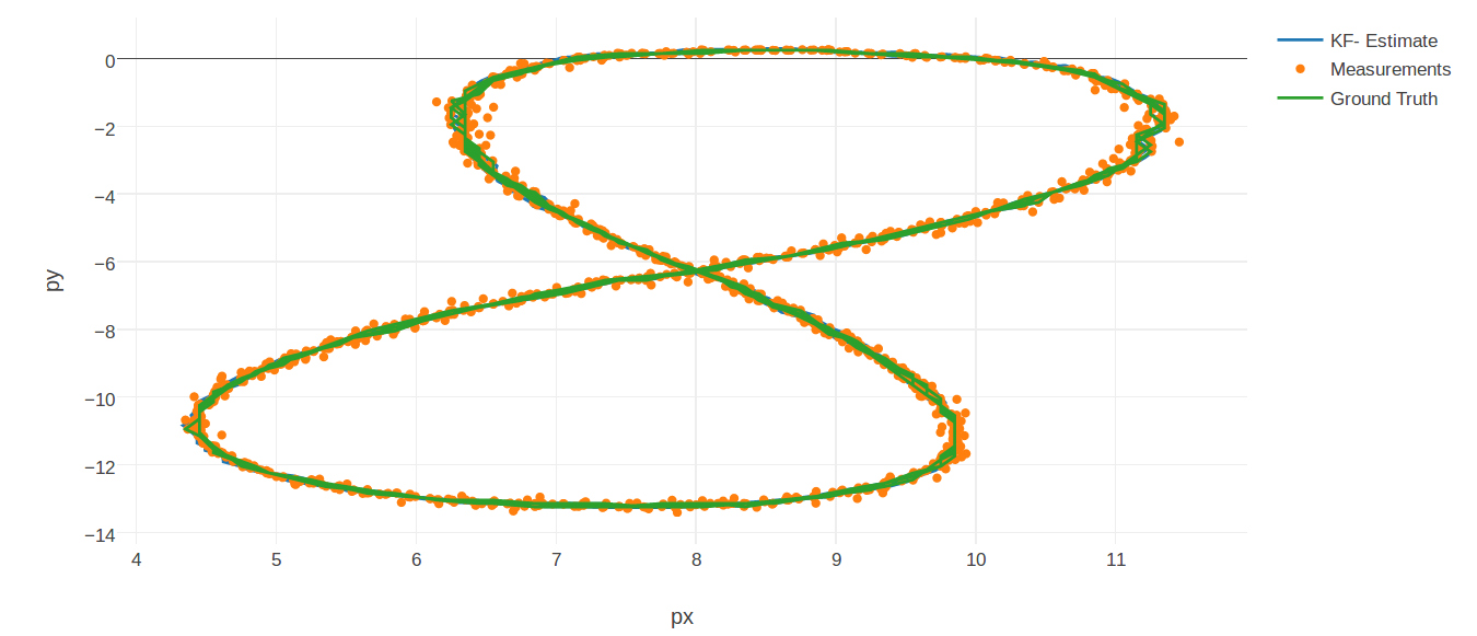
Plotting the lissajous figure using the visualization toolkit generates the following image. This is specifically for the first data set:

As you can see in the visualization, you can barely see the estimate since the ground truth nearly always covers it. The most variation is at the areas where the lissajous figure curves most rapidly. This is not surprising given the nature of the Extended Kalman Filter with the linear nature of its prediction.