TPMplt package

TPMplt package is a tool-kit for building dynamic material model (DMM), as well as for raw data smoothing, adiabatic heating correction, the calculation for constitutive equation.

Installation

Installation from github:

if(! "devtools" %in% installed.packages()) install.packages("devtools")
devtools::install_github("CubicZebra/TPMplt")

Installation from CRAN:

install.packages("TPMplt")

Main functions

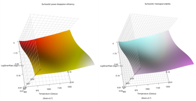
TPMplt is a tool-kit for building the dynmaic materials model (DMM), suggested by Prasad and Gegel, and executing the corresponding visualization. It also provide a feasible approach to calculate the constitutive equation, material constants, as well as all the intermediate fitting plots for reference. The processing-maps can be display not only in 2D using gradient color background superpositioned with contours customarily, but also in two 3D surfaces individually.

Workflow

Kalman smoothing for noise reduction

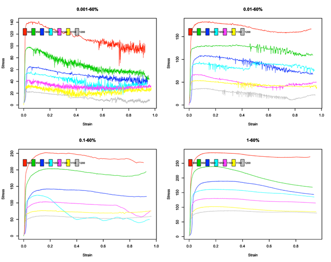
The function KFprocess() can apply Kalman smoothing for all raw data for flow stess-strain curves.

Following figures show the raw data with significant vibration in plastic deformation period:

After using Kalman filter, the curves will be of more clear paths:

Adiabatic heating correction

The phenomenon of adiabatic temperature rise non-negligible, especially in the conditions of low temperatures, high strain rates, or even both. Rationally, before the calculation for the processing maps, adiabatic heating correction should be utilized. The function TCorrect() can implement the automatic correction for this phenomenon. The corrected results will be:

Computation for dynamic material model and output corresponding figures

The function used to build dynamic material model (DMM) for materials is DMMprocess(). This function has two most important arguments: InteractMode and ConsFun. The argument InteractMode control the output of figures and parameters computed for DMM. If the value of ConsFun is TRUE``, the constitutive equation will be calculated then printed out. Additionally, if its value of InteractModeis set asTRUE``` simultaneously, the following figures can be exported one by one:

Related parameters in each intermediate step will be printed out in console as well, when InteractMode is TRUE:

Processing Map Preview

Conventional 2D processing map

After making the model followed with regression, the 2D can be visualized as:

The background in gradient colors informs the stability coefficient $\xi$, while the contours denotes the power dissipation efficiency $\eta$.

3D processing maps

$\xi$ and $\eta$ can also be respectively generated using the 3D plot function. The result will be as:

Operations such as mouse rotation, zoom in and zoom out are also available in this visualization mode. Users can use those operations flexibly, to find out more interesting things which might be difficult to be found out in 2D visualization.

Contact

Author: Chen Zhang

Mail: [email protected]