This repository contains a calibration tool to calibrate a sensor setup consisting of lidars, radars and cameras. Using this extrinsic sensor calibration tool, the sensor poses can be estimated with respect to each other. This code has bindings with Robot Operating System (ROS). For more information, we would like to refer to the ICRA 2019 conference paper (see [1]).
This tutorial explains how to use the multi_sensor_calibration toolbox. It consists of the following main components:
- detector nodes detect the calibration board (see calibration board) for every sensing modality (lidar, monocular/stereo camera, and radar)
- accumulator node collects the detections of the various calibration board locations.
- optimizer node optimizes all sensors poses.
- urdf writer updates the sensors poses in the URDF file.
The code has been developed in Ubuntu 16.04 LTS in combination with ROS Kinetic Kame. Furthermore, the software has been tested on Ubuntu 18.04 LTS in combination with ROS Melodic Morenia.
The following ROS dependencies are present:
    apt-get install ros-<ros_distro>-desktop-full
    apt-get install ros-<ros_distro>-pcl-ros
    apt-get install ros-<ros_distro>-opencv3
    apt-get install ros-<ros_distro>-ros-numpy
    apt-get install ros-<ros_distro>-astuff-sensor-msgs
The following packages need to be installed:
    apt-get install libeigen3-dev
    apt-get install python-rospkg
    apt-get install build-essential
    apt-get install python3-dev
    apt-get install python3-setuptools
    apt-get install libatlas-dev
    apt-get install libatlas3-base
    apt-get install python3-numpy
    apt-get install python3-scipy
    apt-get install python3-pip
    apt-get install python3-matplotlib
    apt-get install python3-yaml
    apt-get install python3-sklearn
    pip3 install rmsd
    pip3 install rospkg
    pip3 install tikzplotlib
Clone our multi_sensor_calibration package to the src folder as well. After that, build catkin workspace:
    git clone https://github.com/tudelft-iv/multi_sensor_calibration.git
    cd <path to catkin_ws folder>
    catkin_make
    source devel/setup.bash
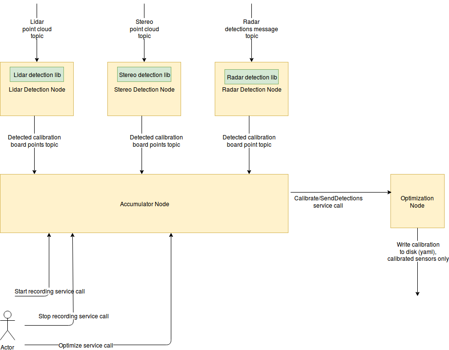
The overview of the components in the calibration tool are visualized in the following figure. Note that in this figure the calibration is performed with a single lidar, radar and stereo camera. The calibration tool can accommodate more sensors. More details on subscribed and published topics for the detectors nodes can be found in detectors.

The next steps need to be performed to calibrate your sensor setup.
For each detector except for the radar detector, the YAML file is used to define the parameters of the detector:
- Lidar Detector: lidar_detector/config/config.yaml
- Stereo Detector: stereo_detector/config/config.yaml
- Mono Detector: mono_detector/config/config.yaml
- Radar detector: configuration is determined as ROS parameters (example here). Specifically, one can specify a min and max range and RCS, as well as define the selection criteria within that range (i.e. choose to select the highest/lowest range/RCS).
Note that we provide some additional information about the detectors in: detectors.
This can be done by:
    rosrun lidar_detector lidar_detector_node
    rosrun radar_detector radar_detector_node
    rosrun stereo_detector stereo_detector_node
    rosrun mono_detector mono_detector_node
For instance, you can find for every node the subscribed and published topics. We recommend you to visualize the published topics to check if the detectors are working (see detectors).
We also provide a launch file with the lidar, camera and radar detector in the package multi_sensor_calibration_launch :
roslaunch multi_sensor_calibration_launch detectors.launch
Note: In case of multiple sensors, multiple instances of the detectors should be launched. This means that topics have to be remapped.
Check the terminal of the accumulator to check status messages.
The accumulator collects all detections from various calibration board locations and prepares the data set with calibration board detections that will be send to the optimizer.
rosrun accumulator accumulator
Alternatively, the launch file can be used:
roslaunch multi_sensor_calibration_launch accumulator.launch
The optimizer python node estimates all sensors poses given the sensors measurements. If your calibration board geometry differs from ours, change it in the python file optimization/src/optimization/calibration_board.py. The python file optimization/src/optimization/config.py contains the information about the sensor setup and specific information about the sensors.
rosrun optimization server.py
The multi_sensor_calibration_launch also contains a launch file that runs the optimizer:
roslaunch multi_sensor_calibration_launch optimizer.launch
The default joint optimization configuration is Fully Connected Pose Estimation (FCPE) (see [1] for more information) and the default reference sensor is Velodyne. The calibration_mode and reference_sensor can be changed in the by setting the following ROS parameters:
    rosparam set /optimizer/calibration_mode <calibration_mode>
    rosparam set /optimizer/reference_sensor <reference_sensor>
For more information on these parameters, see comments the code: see the function joint_optimization in optimization/src/optimization/optimize.py .
Recommendations calibration:
- Position the calibration board in a free space
- Do not hold the calibration board in you hands, since you will affect the radar detections.
To record a new calibration board location:
    rosservice call /accumulator/toggle_accumulate # Start recording
    # Wait until you are happy with the number of recorded detections.
    # In our case we wait 5 to 10 seconds to collect detections.
    rosservice call /accumulator/toggle_accumulate # Stop recording
Check the terminal of the accumulator to check the status of the accumulator. If you are happy with the number of calibration board locations, you can perform the calibration by calling the rosservice call optimize. We recommend to aim for (at least) 10 calibration board locations (see our experiments in [1] for more details) in the field of view of all the sensors.
rosservice call /accumulator/optimize
By this command the accumulated board locations are sent to the optimizer. The accumulator also publishes a visualization_msg::MarkerArray message with all calibration board detections so that these can be visualized in RViz. By visualizing these markers, you can see which detections are sent to the optimizer.
When the optimizer receives the request, all the sensors poses will be computed. You should check the terminal of the optimizer for the output of the optimizer. The optimizer also provides a figure with the optimized results. In this plot, the sensor poses and all detections are visualized.
Other convenient rosservice calls are the save and load service calls. The save rosservice call writes all collected detections of all calibration board locations to a yaml file. The rosservice call is as follows (note that tab completion works):
rosservice call /accumulator/save "data: {data: '<path_to_output_yaml_file>'}"
The rosservice call load read the saved yaml file again:
rosservice call /accumulator/load "data: {data: '<path_to_input_yaml_file>'}"
The outcome is exported to YAML files and launch files in the default results directory:
- YAML files contains the transformation matrix from source to target. This transformation matrix can be used to transform detections from source reference frame to target reference frame.
- Launch files containing the poses of the sensor with respect to parent link. This file contains a ROS static_transform_publisher:
- In order to quickly test the output:
roslaunch results/<sensor>.launch
- In order to quickly test the output:
The URDF_CALIBRATION tool can be used to update your URDF with calibrated values (from YAML). In order to update your robot URDF file with your updated sensor pose, the urdf_calibration node can be used. This node computes the pose of the link_to_update and joint_to_update, you would like to update given a transformation between two reference frames (as defined in the YAML file).
rosrun urdf_calibration urdf_calibration <input_urdf_file> <calibration_urdf_or_yaml_file> <output_urdf_file> <link_to_update> <joint_to_update>
This command needs to be repeated for every sensor. Please note that you should not update the same link and joint multiple times, since otherwise the outcome will not be correct. This problem might occur if your tf tree has sensors with a common parent. As an example, a bash script is provided in the folder multi_sensor_calibration_launch that contains the commands to update our URDF:
./multi_sensor_calibration_launch/scripts/update_prius_urdf.sh
Now we are finished with extrinsic calibration of the sensors of the car. In the next section, we show two examples on how to use the optimizer.
Below, two examples are provided to show the results of our calibration tool. These two examples use provided measurement files so that the user is able to test the optimization.
In the first terminal, you start the accumulator:
rosrun accumulator accumulator
You have to make sure that you run a roscore as well. In the second terminal, you start the optimizer:
rosrun optimization server.py
In the third terminal, go the folder containing our calibration and load the example YAML:
    rosservice call /accumulator/load "data: {data: '<path_to_repository>/accumulator/data/example_data.yaml'}"
    rosservice call /accumulator/optimize
With the FCPE configuration, you should see the following results in the terminal running the optimizer:
-------------------------------------
Optimization terminated successfully!
-------------------------------------
RMSE  velodyne to radar =  0.01460
RMSE  velodyne to left =  0.02386
RMSE  left to radar =  0.02211
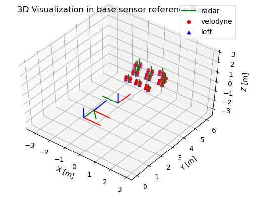
In addition, you will see the following figure appearing:
In the following two examples, we will run the optimizer with csv files as input. The first showcases a basic optimization in which all calibration board detections were succesful. The second showcases what to do when some calibration board detections were unsuccesful.
Go to the folder containing our calibration tool code:
cd optimization/
python3 src/main.py --lidar data/example_data/lidar.csv --camera data/example_data/camera.csv --radar data/example_data/radar.csv --calibration-mode 3 --visualise
You should see the following result, indicating the overall Root Mean Square Error between every two sensors, as well as the 20 largest errors per item, sorted by size:
----------------------------------------------------------------
Optimizing your sensor setup using FPCE
----------------------------------------------------------------
-------------------------------------
Optimization terminated successfully!
-------------------------------------
RMSE  camera1 to lidar1 =  0.01525
    Error per item: {86: 0.038, 87: 0.036, 82: 0.031, 83: 0.031, 74: 0.03, 10: 0.027, 11: 0.027, 96: 0.026, 81: 0.025, 80: 0.024, 85: 0.022, 75: 0.021, 103: 0.021, 68: 0.021, 70: 0.021, 84: 0.019, 93: 0.019, 37: 0.019, 7: 0.018, 18: 0.018}
RMSE  lidar1 to radar1 =  0.01427
    Error per item: {24: 0.033, 25: 0.027, 1: 0.026, 2: 0.021, 12: 0.021, 0: 0.02, 26: 0.019, 23: 0.016, 5: 0.015, 6: 0.015, 22: 0.012, 15: 0.012, 19: 0.011, 21: 0.01, 18: 0.009, 8: 0.009, 11: 0.008, 4: 0.008, 10: 0.008, 28: 0.007}
RMSE  camera1 to radar1 =  0.02111
    Error per item: {24: 0.046, 25: 0.038, 1: 0.031, 23: 0.031, 0: 0.031, 12: 0.028, 6: 0.024, 26: 0.024, 21: 0.021, 2: 0.021, 11: 0.021, 15: 0.02, 5: 0.02, 20: 0.019, 17: 0.018, 22: 0.018, 28: 0.016, 4: 0.013, 9: 0.013, 27: 0.012}
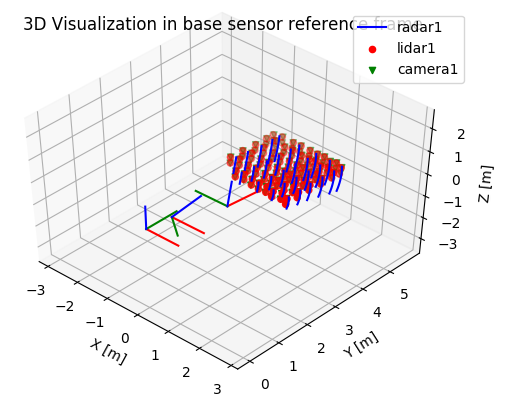
In addition, you will see the following figure, with all 29 calibration board locations in a grid:
In the following example, the fifth and sixth radar detections have been translated, as well as the first and final set of four lidar detections. Run the following command:
python3 src/main.py --lidar data/example_data/lidar_with_error.csv --camera data/example_data/camera.csv --radar data/example_data/radar_with_error.csv --calibration-mode 3 --visualise --sensors_to_number radar1 --plot_correspondence radar1 lidar1
You should see the following result, indicating the overall Root Mean Square Error between every two sensors, as well as the 20 largest errors per item, sorted by size:
----------------------------------------------------------------
Optimizing your sensor setup using FPCE
----------------------------------------------------------------
-------------------------------------
Optimization terminated successfully!
-------------------------------------
RMSE  camera1 to lidar1 =  0.99894
    Error per item: {112: 3.69, 114: 3.677, 113: 3.649, 115: 3.639, 0: 3.611, 2: 3.608, 3: 3.578, 1: 3.578, 97: 0.469, 99: 0.468, 85: 0.458, 87: 0.453, 67: 0.445, 65: 0.444, 23: 0.443, 41: 0.441, 21: 0.44, 43: 0.437, 96: 0.432, 98: 0.429}
RMSE  lidar1 to radar1 =  1.36084
    Error per item: {6: 4.79, 28: 3.612, 0: 3.51, 5: 1.267, 21: 0.609, 16: 0.567, 20: 0.54, 10: 0.524, 15: 0.5, 19: 0.484, 24: 0.484, 9: 0.448, 14: 0.434, 18: 0.417, 4: 0.408, 8: 0.374, 23: 0.369, 17: 0.362, 13: 0.354, 3: 0.323}
RMSE  camera1 to radar1 =  0.94077
    Error per item: {6: 4.884, 5: 1.139, 21: 0.186, 20: 0.175, 18: 0.171, 19: 0.17, 16: 0.168, 14: 0.159, 15: 0.158, 17: 0.156, 10: 0.154, 13: 0.151, 9: 0.149, 11: 0.145, 8: 0.144, 0: 0.136, 24: 0.136, 4: 0.134, 7: 0.132, 3: 0.125}
The overall RMSE is high, and the error per item shows that only a few detections are causing it. In the camera to radar correspondence, there is a high error on the 5th and 6th correspondence. In the lidar to radar correspondence, it is the 5th, 6th as well as the first and final. For the camera to lidar, it is the 112th to 115th location, as well as the 0th to 3rd: as both camera and lidar detections come in sets of four, this means it's the first and final set of four lidar to camera correspondences.
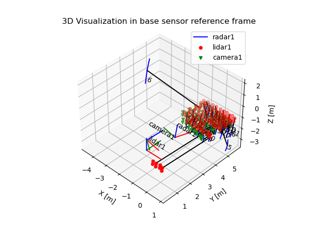
The visualisation now also shows the index of the radar detections, along with the correspondence between each radar detection and lidar detection. This further shows that the culprits are two faulty radar detections and two faulty sets of lidar detections.
Loading a YAML file (found here) that defines which boards to ignore is done as follows:
python3 src/main.py --lidar data/example_data/lidar_with_error.csv --camera data/example_data/camera.csv --radar data/example_data/radar_with_error.csv --ignore_file data/example_data/ignored_measurements.yaml --calibration-mode 3 --visualise --sensors_to_number radar1 --plot_correspondence radar1 lidar1
Which results in a lower error and a better calibration:
----------------------------------------------------------------
Optimizing your sensor setup using FPCE
----------------------------------------------------------------
-------------------------------------
Optimization terminated successfully!
-------------------------------------
RMSE  camera1 to lidar1 =  0.01545
    Error per item: {82: 0.038, 83: 0.036, 78: 0.031, 79: 0.031, 70: 0.03, 6: 0.027, 7: 0.027, 92: 0.026, 77: 0.025, 76: 0.024, 81: 0.022, 64: 0.021, 66: 0.021, 71: 0.021, 99: 0.021, 89: 0.02, 80: 0.019, 33: 0.019, 14: 0.018, 3: 0.018}
RMSE  lidar1 to radar1 =  0.01413
    Error per item: {21: 0.033, 22: 0.026, 0: 0.026, 1: 0.021, 9: 0.02, 23: 0.019, 20: 0.017, 19: 0.012, 12: 0.011, 16: 0.01, 18: 0.01, 7: 0.009, 15: 0.009, 3: 0.008, 8: 0.008, 5: 0.008, 4: 0.007, 11: 0.007, 6: 0.007, 13: 0.006}
RMSE  camera1 to radar1 =  0.02102
    Error per item: {22: 0.047, 23: 0.037, 21: 0.033, 0: 0.032, 1: 0.031, 10: 0.026, 24: 0.023, 9: 0.02, 2: 0.02, 19: 0.02, 13: 0.019, 20: 0.019, 15: 0.019, 18: 0.018, 26: 0.018, 4: 0.014, 25: 0.013, 7: 0.012, 8: 0.011, 5: 0.01}
Note that ignoring the largest errors will always reduce the RMSE, and as such a lower error does not directly translate into a better calibration. Use the above only for removing outliers.
The current setup allows for multiple sensors of the same modality. In the following example, 3D radar detections have been simulated by computing their expected position using the camera detections. The following command optimizes four sensors at once (of which two radar), using MPCE:
python3 src/main.py --lidar data/example_data/lidar.csv --camera data/example_data/camera.csv --radar data/example_data/radar.csv --radar data/example_data/radar_3D.csv --calibration-mode 2 --visualise
As a result, you get the error between every set of sensors. As radar_3D.csv was added second, it is referred to as radar2 in the bottom output.
----------------------------------------------------------------
Optimizing your sensor setup using MCPE
----------------------------------------------------------------
-------------------------------------
Optimization terminated successfully!
-------------------------------------
RMSE  camera1 to lidar1 =  0.01525
    Error per item: {86: 0.038, 87: 0.036, 82: 0.031, 83: 0.031, 74: 0.03, 10: 0.028, 11: 0.027, 96: 0.026, 81: 0.025, 80: 0.024, 85: 0.022, 75: 0.021, 68: 0.021, 70: 0.021, 103: 0.021, 84: 0.019, 93: 0.019, 37: 0.019, 7: 0.019, 18: 0.019}
RMSE  lidar1 to radar1 =  0.01965
    Error per item: {24: 0.039, 1: 0.037, 25: 0.036, 2: 0.028, 12: 0.028, 0: 0.026, 26: 0.026, 6: 0.025, 5: 0.024, 21: 0.021, 23: 0.019, 11: 0.019, 10: 0.016, 22: 0.015, 16: 0.014, 4: 0.013, 7: 0.013, 19: 0.012, 9: 0.012, 28: 0.011}
RMSE  radar2 to lidar1 =  0.01276
    Error per item: {21: 0.023, 17: 0.022, 20: 0.019, 2: 0.017, 25: 0.016, 19: 0.016, 16: 0.016, 23: 0.015, 1: 0.014, 0: 0.013, 24: 0.013, 11: 0.013, 12: 0.012, 18: 0.012, 22: 0.011, 26: 0.011, 27: 0.01, 15: 0.01, 6: 0.01, 9: 0.01}
RMSE  camera1 to radar1 =  0.02642
    Error per item: {24: 0.052, 25: 0.047, 1: 0.042, 0: 0.038, 23: 0.034, 6: 0.034, 12: 0.034, 11: 0.031, 26: 0.03, 17: 0.029, 5: 0.029, 21: 0.028, 2: 0.026, 22: 0.02, 28: 0.02, 10: 0.02, 20: 0.019, 15: 0.019, 16: 0.018, 4: 0.018}
RMSE  camera1 to radar2 =  0.00271
    Error per item: {24: 0.005, 23: 0.005, 22: 0.005, 12: 0.004, 0: 0.004, 28: 0.004, 27: 0.004, 26: 0.004, 25: 0.004, 5: 0.003, 4: 0.003, 3: 0.003, 2: 0.003, 1: 0.003, 10: 0.002, 9: 0.002, 8: 0.002, 7: 0.002, 6: 0.002, 16: 0.001}
RMSE  radar2 to radar1 =  0.02642
    Error per item: {24: 0.052, 25: 0.047, 1: 0.042, 0: 0.038, 23: 0.034, 6: 0.034, 12: 0.034, 11: 0.031, 26: 0.03, 17: 0.029, 5: 0.028, 21: 0.028, 2: 0.026, 22: 0.02, 28: 0.02, 10: 0.02, 20: 0.02, 15: 0.019, 16: 0.018, 4: 0.018}
Note that as radar2 was simulated using the 3D data from camera1, the error camera1 to radar2 is practically zero.
Yes, you can. The only requirement is that you have at least one 3D sensor. In that case, you need to start a detector for every sensor (see detectors). The accumulator needs to know which topics need to be recorded. The ROS topics can be set using sensors_topic which is a ROS parameter.
Yes, you should be able to do it, however there are some limitations and it has not been tested extensively. The accumulator returns point cloud with NaNs in case the detector didn't detect something. The optimizer is able to deal with missing detections of a sensor.
For that, currently you need to use:
- At least one sensor should be able to see all calibration board locations. This means that for this sensor all calibration board locations are visible (aka all mu should be equal to true). Choose this sensor as reference sensor. A lidar is often a good choice as reference sensor since it has a (often) 360 degrees sensing.
- mode = 'remove_detections' in remove_outlier_detections. This can be found in the function get_sensor_setup() in src/optimization/config.py for the python script: src/main.py. For the ROS node, it is a ROS parameter with the name outlier_removal.
The toolbox contains two methods to determine the correspondences. The first method is equivalent to [2], in which the points in lidar and camera are labeled as top-left, top-right, bottom-left and bottom-right. The second method, which is the recommended method, is based on reordering the circle center detections for each calibration board location based on a 'reference sensor'. For that, the initial relative sensor pose is determined using the centroids of all calibration board detections. After that, the detections are reordered to match the detections in the reference sensor by assigned to closest detection to each detection in the 'reference sensor'.
(Additionally, the optimization configurations are also able to determine the correspondences during optimization, however it is not recommended since it takes more time.)
- Test option to calibrate sensors with partial overlapping field of view.
- Include option to compute radar to radar errors in all configuration.
- Remove PCL warnings in lidar_detector.
GPL license. In every package, you can find the license file with the details.
We would like to thank to authors of [2] for their work on lidar to stereo camera calibration. In order to be able to deal multiple sensors and with multiple calibration board locations, we have decided to re-implement the stereo_detector and lidar_detector.
[2] Guindel, C., Beltrán, J., Martín, D., & García, F. (2017, October). Automatic extrinsic calibration for lidar-stereo vehicle sensor setups. In 2017 IEEE 20th International Conference on Intelligent Transportation Systems (ITSC) (pp. 1-6). IEEE.
- Joris Domhof
- Ronald Ensing
- Julian F.P. Kooij
- Dariu M. Gavrila
Intelligent Vehicles group, Cognitive Robotics Department, Delft University of Technology, the Netherlands
Please cite the following paper if you use our code: [1] Joris Domhof, Julian F. P. Kooij and Dariu M. Gavrila, An Extrinsic Calibration Tool for Lidar, Camera and Radar, ICRA 2019 conference.


