记录点云SemanticKITTI论文阅读记录
纯图像分割方法:可以考虑用在投影图上面,也可以考虑用在多体素分割的上面,用来提升不同大小的物体的分割

# 注意力部分的相关代码
if pred is None:
    pred = cls_out
    aux = aux_out
elif s >= 1.0:
    # downscale previous
    pred = scale_as(pred, cls_out)
    pred = attn_out * cls_out + (1 - attn_out) * pred
    aux = scale_as(aux, cls_out)
    aux = attn_out * aux_out + (1 - attn_out) * aux
else:
    # s < 1.0: upscale current
    cls_out = attn_out * cls_out
    aux_out = attn_out * aux_out

    cls_out = scale_as(cls_out, pred)
    aux_out = scale_as(aux_out, pred)
    attn_out = scale_as(attn_out, pred)

    pred = cls_out + (1 - attn_out) * pred
    aux = aux_out + (1 - attn_out) * aux

# ocrnet.py 产生logit_attn的代码
def _fwd(self, x):
    x_size = x.size()[2:]

    _, _, high_level_features = self.backbone(x)
    cls_out, aux_out, ocr_mid_feats = self.ocr(high_level_features)
    # 产生相关的注意力
    attn = self.scale_attn(ocr_mid_feats)

    aux_out = Upsample(aux_out, x_size)
    cls_out = Upsample(cls_out, x_size)
    attn = Upsample(attn, x_size)

    return {'cls_out': cls_out,
            'aux_out': aux_out,
            'logit_attn': attn}

'''
self.scale_attn 来源
可以看到是conv+bn+relu+sigmoid的注意力操作
'''
def make_attn_head(in_ch, out_ch):
    bot_ch = cfg.MODEL.SEGATTN_BOT_CH
    if cfg.MODEL.MSCALE_OLDARCH:
        return old_make_attn_head(in_ch, bot_ch, out_ch)

    od = OrderedDict([('conv0', nn.Conv2d(in_ch, bot_ch, kernel_size=3,
                                          padding=1, bias=False)),
                      ('bn0', Norm2d(bot_ch)),
                      ('re0', nn.ReLU(inplace=True))])

    if cfg.MODEL.MSCALE_INNER_3x3:
        od['conv1'] = nn.Conv2d(bot_ch, bot_ch, kernel_size=3, padding=1,
                                bias=False)
        od['bn1'] = Norm2d(bot_ch)
        od['re1'] = nn.ReLU(inplace=True)

    if cfg.MODEL.MSCALE_DROPOUT:
        od['drop'] = nn.Dropout(0.5)

    od['conv2'] = nn.Conv2d(bot_ch, out_ch, kernel_size=1, bias=False)
    od['sig'] = nn.Sigmoid()

    attn_head = nn.Sequential(od)
    # init_attn(attn_head)
return attn_head输入两个不同分辨率的图像,网络学习不同物体在相应分支上的权重
- 多尺度分割,目前分割的效果是Cityscapes Dataset SOTA层次的模型
- 模型计算量、参数量都十分巨大,很难迁移

class PSA_p(nn.Module):
    def __init__(self, inplanes, planes, kernel_size=1, stride=1):
        super(PSA_p, self).__init__()

        self.inplanes = inplanes
        self.inter_planes = planes // 2
        self.planes = planes
        self.kernel_size = kernel_size
        self.stride = stride
        self.padding = (kernel_size-1)//2

        self.conv_q_right = nn.Conv2d(self.inplanes, 1, kernel_size=1, stride=stride, padding=0, bias=False)
        self.conv_v_right = nn.Conv2d(self.inplanes, self.inter_planes, kernel_size=1, stride=stride, padding=0, bias=False)
        self.conv_up = nn.Conv2d(self.inter_planes, self.planes, kernel_size=1, stride=1, padding=0, bias=False)
        self.softmax_right = nn.Softmax(dim=2)
        self.sigmoid = nn.Sigmoid()

        self.conv_q_left = nn.Conv2d(self.inplanes, self.inter_planes, kernel_size=1, stride=stride, padding=0, bias=False)   #g
        self.avg_pool = nn.AdaptiveAvgPool2d(1)
        self.conv_v_left = nn.Conv2d(self.inplanes, self.inter_planes, kernel_size=1, stride=stride, padding=0, bias=False)   #theta
        self.softmax_left = nn.Softmax(dim=2)

        self.reset_parameters()
        '''
            具体请见github代码
'''- 极化滤波( Polarized filtering):在通道和空间维度保持比较高的resolution(在通道上保持C/2的维度,在空间上保持[H,W]的维度 ),这一步能够减少降维度造成的信息损失;
- 增强(Enhancement):组合非线性直接拟合典型细粒度回归的输出分布。
- 代码比较简单易懂
主要思路+解读1
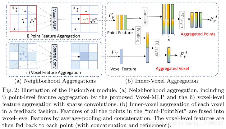
左边刻画的是Neighborhood aggregation
右边刻画的是Inner-voxel aggregation
主要是体素融合(依靠稀疏3D卷积spconv)和点云级别的邻点特征聚合(这里是否可以考虑单个体素的梯度信息,用来刻画物体表面的一个信息,感觉可以比较好的来刻画一个物体)
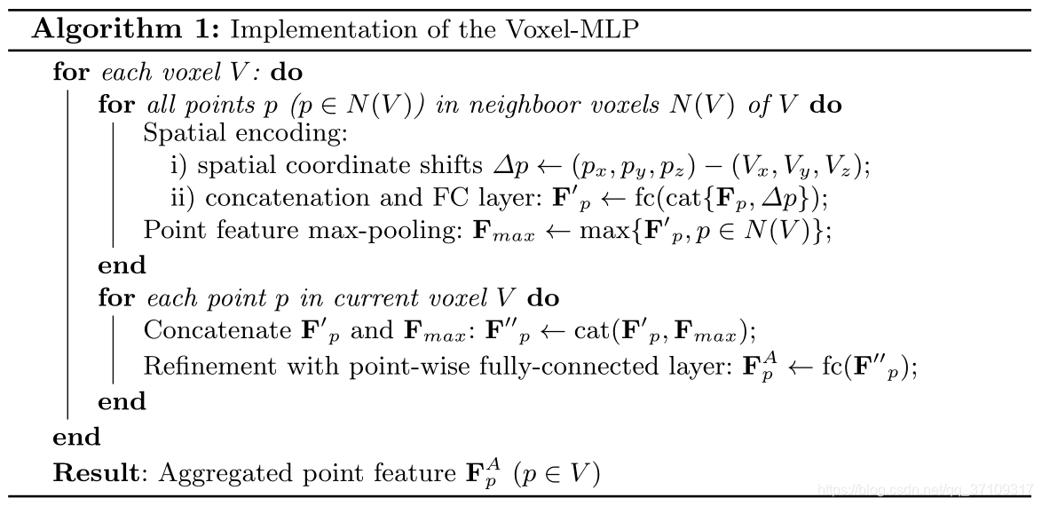
- 对于每一个体素,去用hash表索引这个点所在体素的身边的体素的点(针对特定的kernel_size,包括自己)
- 每个点去做空间偏移,即
$\triangle p=(x,y,z){point}-(x',y',z'){voxel}$
- Feature of Point(
$F_p$ ) concat with$\triangle p$ →Fc - MaxPooling
$F_{max}=max{F'_p, p{\in}N(V)}$ - $cat(F'p,F{max})$→$Fc$→$F^A_p$(更新单点的特征)
Point Interpolation(PointNet code) (上采样,by PointNet++ 解读 code)
论文中描述错误,插值方法应该引用自PointNet++,总而言之,论文PointNet和PointNet++很值得仔细看一看
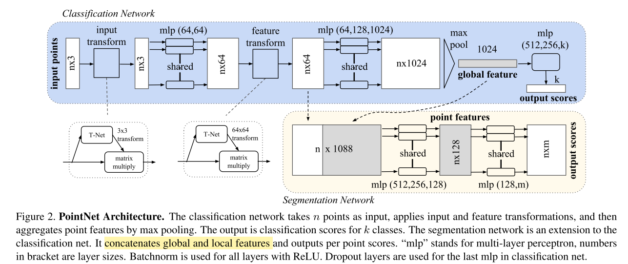
PointNet的代码和结构的图没有差别,主要就是根据Fc去映射特征并且使用最大池化+Fc得到一个[batchsize, kxk]的特征,然后再去+eye(k)最后reshape →[batchsize, k, k]作为一个类似于旋转的变换对齐矩阵,矩阵来自数据自身

PointNet++的插值方法,使用CUDA自定义编写的插值,知乎上这么描述:如果将多个这样的处理模块级联组合起来,PointNet++就能像CNN一样从浅层特征得到深层语义特征。对于分割任务的网络,还需要将下采样后的特征进行上采样,使得原始点云中的每个点都有对应的特征。这个上采样的过程通过最近的k个临近点进行插值计算得到
Semantic KITTI: The Semantic KITTI dataset is a new large-scale LiDAR point cloud dataset in driving scenes. It has 22 sequences with 19 valid classes, and each scan contains 10–13k points in a large space of 160m×160m×20m. We use Sequences 0–7 and 9–10 as the training set (in total 19k frames), Sequence 8 (4k frames) as the validation set, and the remaining 11 sequences (20k frames) as the test set. Different from other point cloud datasets, LiDAR points are distributed irregularly in a large 3D space. There are many small objects with only a few points and the points are very sparse in the distance. All these make it challenging for semantic segmentation of the large-scale LiDAR point clouds.
- When compared to existing voxel networks, FusionNet can predict point-wise labels and avoid those ambiguous/wrong predictions when a voxel has points from different classes(可以区分更加细粒度的特征:由于点云的嵌入).
- When compared to the popular PointNets and point-based convolutions, FusionNet has more effective feature aggregation oper- ations (including the efficient neighborhood-voxel aggregations and the fine- grain inner-voxel point-level aggregations). These operations help produce better accuracy for large-scale point cloud segmentation(体素聚合依靠稀疏卷积 & 体素内部聚合??方法是什么).
- FusionNet takes full advantage of the sparsity property to reduce its memory footprint. For instance, it can take more than one million points in training and use only one GPU to achieve state-of-the-art accuracy(内存的高效).
- 三维数据本身具有复杂性,图像可以简单的RGB数组
- 三维数据可以表示为点云、Mesh(计算机图形学,适合渲染建模)、Voxel(体素)、MultiView(RGB-D)
- 传感器最原始的数据,表达简单,非常适合端到端的学习
- Mesh需要选择大小、多边形
- 体素需要确定分辨率
- 图像需要角度,一个视角,表达不全面
- 计算代码很大,$O(N^3)$
- 体素量化有误差
- 如果分辨率很大,那么很多都是空白的
- 损失3D的信息
- 决定投影的角度
- 手工的特征限制了特征的表示
- 无序性,置换不变性 (使用对称函数解决,MeanPooling、MaxPooling)
- 最初的最大池化可能只能取得边界的信息,平均池化可能只能取得中心的
- 先升维,这样子得到的信息是冗余的空间,这样综合起来就可以避免信息的丢失
- 实验中表明,最大池化是一种效果比较好的操作
- PointNet要么是对单个点在操作,要么是针对全局的点操作,没有一个局部的概念(local context),缺少一个平移不变性的特征
- 针对这些问题,提出了PointNet++,在局部使用PointNet
- 选取小区域 平移到局部坐标系 得到一个新的点Point(X,Y,F),其中F是小区域的几何形状信息
- 重复操作,得到一个新的点的集合(点一般会变少),得到高维的特征,有点类似于卷积神经网络的操作
- 再通过upsample的方法恢复(3D插值)
PointNet++的局部操作会被采样率的不均匀影响,应该要学习不同区域大小的特征去得到一个鲁棒的模型
点云处理——声音有点糊,但是值得好好听一下里面的笼统的介绍
- 点云滤波(filtering)
- 检测和移除点云中的噪声或不感兴趣的点
- 分类
- 基于统计信息(statisca I-based)
- 基于领域(ne ighbor -based)
- 基于投影(project ion-based)
- 基于信号处理(singal process ing based)
- 基于偏微分方程(PDEs-based)
- 其他方法: voxel grid fit ler ing,quadtree-based, etc.
- 常用方法
- 基于体素(voxel grid)
- 移动平均最小二乘(Moving Least Squares)
- 点云匹配(point cloud registration): .
- 估计两帧或者多帧点云之间的rigid body transformation信息,将所有帧的点云配准在同一个坐标系。
- 分类
- 初/粗匹配:适用于初始位姿差别大的两帧点云
- 精匹配:优化两帧点云之间的变换
- 全局匹配:通常指优化序列点云匹配的误差,如激光SLAM,两帧之间匹配,全局匹配
- 常用方法
- 基于Iterative Closest Point (ICP)的方法
- 基于特征的匹配方法
- 深度学习匹配方法
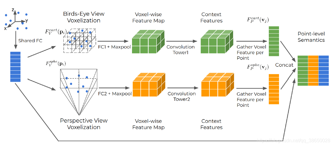
- 算法能够利用相同LiDAR的点云数据中的鸟瞰图和透视图之间的互补信息
- 动态体素化消除了对每一个体素采样预定义点数的需要,这意味着每一个点可以被模型使用,从而减少信息损失
//#define DEBUG
const int THREADS_PER_BLOCK_NMS = sizeof(unsigned long long) * 8;
const float EPS = 1e-8;
struct Point {
// 优秀的工程师都有自己的cuda自定义包能力,
// 的确有时间可以学习一下
from spconv.utils import VoxelGenerator
self.voxel_generator = VoxelGenerator(
voxel_size=voxel_generator_cfg.VOXEL_SIZE,
point_cloud_range=cfg.DATA_CONFIG.POINT_CLOUD_RANGE,
max_num_points=voxel_generator_cfg.MAX_POINTS_PER_VOXEL
)
'''
用到了spconv自带的体素构造器,但是应该基本的
思路和python写的是一样的,所以没什么必要调用
'''Github(代码未开源)
Semantic segmentation of point clouds is a key component of scene understanding for robotics and autonomous driving. In this paper, we introduce TORNADO-Net - a neural network for 3D LiDAR point cloud semantic segmentation. We incorporate a multi-view (bird-eye and range) projection(使用多视角:鸟瞰图+投影图) feature extraction with an encoder-decoder ResNet architecture with a novel diamond context block. Current projection-based methods do not take into account that neighboring points usually belong to the same class. To better utilize this local neighbourhood information and reduce noisy predictions, we introduce a combination of Total Variation,Lovasz-Softmax, and Weighted Cross-Entropy losses(言下之意是Lovasz-Softmax Loss可以避免邻点属于一个类的问题). We also take advantage of the fact that the LiDAR data encompasses 360 degrees field of view and uses circular padding. We demonstrate state-of-the-art results on the SemanticKITTI dataset and also provide thorough quantitative evaluations and ablation results.
The voxel size of the PPL block was set to


"""
TVLoss2D示例代码
"""
import torch
import torch.nn as nn
from torch.autograd import Variable

class TVLoss(nn.Module):
    def __init__(self,TVLoss_weight=1):
        super(TVLoss,self).__init__()
        self.TVLoss_weight = TVLoss_weight

    def forward(self,x):
        batch_size = x.size()[0]
        h_x = x.size()[2]
        w_x = x.size()[3]
        count_h = self._tensor_size(x[:,:,1:,:])
        count_w = self._tensor_size(x[:,:,:,1:])
        h_tv = torch.pow((x[:,:,1:,:]-x[:,:,:h_x-1,:]),2).sum()
        w_tv = torch.pow((x[:,:,:,1:]-x[:,:,:,:w_x-1]),2).sum()
        return self.TVLoss_weight*2*(h_tv/count_h+w_tv/count_w)/batch_size

    def _tensor_size(self,t):
        return t.size()[1]*t.size()[2]*t.size()[3]

def main():
    # x = Variable(torch.FloatTensor([[[1,2],[2,3]],[[1,2],[2,3]]]).view(1,2,2,2), requires_grad=True)
    # x = Variable(torch.FloatTensor([[[3,1],[4,3]],[[3,1],[4,3]]]).view(1,2,2,2), requires_grad=True)
    # x = Variable(torch.FloatTensor([[[1,1,1], [2,2,2],[3,3,3]],[[1,1,1], [2,2,2],[3,3,3]]]).view(1, 2, 3, 3), requires_grad=True)
    x = Variable(torch.FloatTensor([[[1, 2, 3], [2, 3, 4], [3, 4, 5]], [[1, 2, 3], [2, 3, 4], [3, 4, 5]]]).view(1, 2, 3, 3),requires_grad=True)
    addition = TVLoss()
    z = addition(x)
    print(x)
    print(z.data)
    z.backward()
    print(x.grad)

if __name__ == '__main__':
    main()

"""
    SqueezeSegV3、SalsaNext的代码基本是一个模板
    里面有KNN、CRF的代码,可以用来做postprocrss
"""Github 跟SalsaNext也是一套代码
算法,具体可以参见代码
class KNN(nn.Module):
  def __init__(self, params, nclasses):
    super().__init__()
    ...

  def forward(
        self,
        proj_range,
        unproj_range,
        proj_argmax,
        px,
        py
    ):
    ''' Warning! Only works for un-batched pointclouds.
        If they come batched we need to iterate over the batch dimension or do
        something REALLY smart to handle unaligned number of points in memory
    '''
    return knn_argmax_out
"""
(i)S是搜索窗口的大小;
(ii)k是最近邻的数量;
(iii)截止值是k的最大允许范围差;
(iv)高斯逆数。
"""


在论文中,high-rank context可以分为三个维度,即高度(height)、宽度(width)和深度(depth),其中所有三个片段都是低秩的。然后我们使用这些片段建立完整的high-rank context。这种分解-聚合策略(decomposite-aggregate strategy)从不同的角度解决了低秩约束下的高秩问题。三个rank-1的核(3×1×1,1×3×1和1×1×3)用于在所有三维中生成这些低秩编码。然后,Sigmoid函数对卷积结果进行调整,并为每个维度生成权重,其中基于不同视图的rank-1的张量来挖掘共生的上下文信息。将所有三个低秩激活聚合起来,得到表示完整的上下文特征的总和.

3D-MiniNet: Learning a 2D Representation from Point Clouds for Fast and Efficient 3D LIDAR Semantic Segmentation

SalsaNext: Fast, Uncertainty-aware Semantic Segmentation of LiDAR Point Clouds for Autonomous Driving
用到了语义分割的数据增强方法,比如scale+crop
TensorFlow里面tf.math.unsorted_segment_max的功能和torch_scatter.scatter_max是一样的,其实也可以用tf来构造项目
代码未开源
文章提供了一种数据增强的实用方法,可以作为点云在不同的voxel和range-view情况下特征嵌入的一种方法,不过还是得看spconv是否支持,下采样过程中的确有些东西很难控制,特征融合需要很细节的单步调试

All three views have shortcomings. (a) point-based: the points are irregular, which makes finding the neighbors of a point inefficient. (b) voxel-based: voxelization brings quantization loss, and the computation grows cubicly when resolution increases. (c) range-based: range-image distorts physical dimensions because of spherical projection

除了输入的数据,猜想V2P、P2V、R2P、P2R基本都是一个坐标层面的索引,由于point的操作是比较控制上采样的,应该是可以以grid_size//2,grid_size//4等来对low-resolution的图片进行一个feature-embedding,然后进行分割,从整体来看应该不是很难

模型的结构,理解来看应该是取得某个点在体素和投影的特征(unproject),然后使用MLP+softmax来做一个注意力的机制,然后做一个特征融合,再project回去,做一个特征的融合(GFM,Gated Fusion Module,门控注意力机制)
Inspired by past mixbased approaches, we proposed the instance mix to cope with the imbalanced class problem for lidar semantic segmentation. Empirically, the network can predict less frequent objects more accurately if such objects are allowed to repeated in the scene. Motivated by this discover, we extract the rare-class object instances(eg.bicycles, vehicles) from each frame of the training set into a mini sample library. During the training, the samples are randomly selected from the mini-sample pool equally by category. Then, random scaling and rotation will be acted on these samples. To ensure a close fit with reality, we randomly placed the objects above the ground-class points. Finally, some new rare objects from other scenes are “pasted” to the current training scenes, for simulating objects in various environments.
Note that, our result uses the instance CutMix augmentation, and voxel resolution is set to 0.05m, but without extra tricks
Both range and voxel branch are Unet-like architecture with a stem, four down-sampling and four up-sampling stages, and the dimensions of these 9 stages are 32, 64, 128, 256, 256, 128, 128, 64, 32(dimension比较低,估计这个样子可以保持比较大的batchsize),respectively. For range branch, the input range-image size is 64 × 2048 on SemanticKITTI dataset, and 32 × 2048 as initial size for nuScenes dataset, then resized to 64×2048 to keep the same as SemanticKITTI. As for voxel branch, the voxel resolution is 0.05m for the experiments. For point branch, it consists of four per-point MLPs with dimensions: 32, 256, 128, 32.
We employ the commonly used cross-entropy(估计用了instance cutmix数据增强,因此就使用simple-cross-entopy了 as loss in training. Our RPVNet is trained from scratch in an end-to-end manner with the ADAM or SGD optimizer. For the SemanticKITTI dataset, the model uploaded to the leaderboard was trained with SGD, batch size 12(轻量级的网络换来的较可观的batchsize), learning rate 0.24 for 60 epochs(这个数据集似乎就是不需要跑特别多的epochs) on 2 GPUs, which is kept the same as SPVCNN for fair comparison. This setup takes around 100 hours on 2 Tesla V100 GPUs
可以用来学习一下BEV具体是怎么操作的

out_data_dim = [len(pt_fea), self.grid_size[0], self.grid_size[1], self.pt_fea_dim]
out_data = torch.zeros(out_data_dim, dtype=torch.float32).to(cur_dev)
out_data[unq[:, 0], unq[:, 1], unq[:, 2], :] = processed_pooled_data
out_data = out_data.permute(0, 3, 1, 2)
"""
    参考代码很简单的就可以看明白,其实BEV类似于Point2Voxel,都是一个索引的操作
    区别在于Voxel是SparseTensor&有XYZ三轴维度,BEV是torch.Tensor&只需要XY
"""
主要是阐述不同的视图有不同的作用,需要一个融合

其中(b)就是对Assertion的阐述,不同的分支预测,如果两个分支预测的结果相同,那么代表结果可信;如果两个分支的结果不同,那么就需要重新对特征进行衡量

感觉是用来衡量一个物体的形状分布之类的,主要的难度还是在于坐标给定的物体并不是给定物体的坐标,更加深层的应该是在提取物体的轮廓

KD-Tree是怎么解决临近点搜索这种复杂度爆炸高的方法的
KdTree(也称k-d树)是一种用来分割k维数据空间的高维空间索引结构,其本质就是一个带约束的二叉搜索树,基于KdTree的近似查询的算法可以快速而准确地找到查询点的近邻,经常应用于特征点匹配中的相似性算法。
Sparse Single Sweep LiDAR Point Cloud Segmentation via Learning Contextual Shape Priors from Scene Completion
Gihub
Voxel+Point

从图上来看,整体就是核心模型是一个UNet,然后辅助了一些Point-Voxel的分支

看图直观的感觉是使用了PixelShuffle来作为上采样的方式,(b)相当于用KNN做一个几何形状的refine,其实有点类似于一个点云补全(有做一个先验的预测的影子)

从描述来看,似乎要使用多帧的信息来做一个特征的具象化,避免一个物体缺失的问题,具体得参照代码来看
def extract_coord_features(t):
    device = t.device
    channels = int(t.shape[1])
    coords = torch.sum(torch.abs(t), dim=1).nonzero().type(torch.int32).to(device)
    features = t.permute(0, 2, 3, 4, 1).reshape(-1, channels)
    features = features[torch.sum(torch.abs(features), dim=1).nonzero(), :]
    features = features.squeeze(1)
    assert len(coords) == len(features)

    return coords, features
"""
    用来做3D的融合非常合适,这样就可以避免shape不同的问题了
"""(AF)2-S3Net: Attentive Feature Fusion with Adaptive Feature Selection for Sparse Semantic Segmentation Network

模型结构图,更加直观的感觉是使用不同尺度的Conv层然后做了一个注意力,由于代码没有开源,很多细节的地方只能大概理解
"""
geo-aware anisotrophic loss
开源的代码部分并没有这个loss的代码,但是可以通过pad直接去弄
"""大概是意思就是单个点和身边的点去做一个异或操作,核心是为了促使一个点和身边的点尽量的相近