Beam-load-calculation

Calculation of the load of the beam number 49.

The program interface is presented below. There is also a console representation of the program operation.

visual

console

An example of a manual calculation is presented as a docx file at the root of the project, also here.

REPORT Initial data L = 1m; F1 = 2kN; F2 = 3kN; q = 5kN/m.

Rice. 1. Given scheme.

Payment

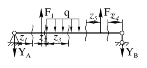
1. Determination of the support reactions for the scheme in Fig. 2 Let us compose the equations of static equilibrium. ∑Fy = F1 + F2 - q 0.3m - YA - YB = 0; ∑MA = F1 0.25m + F2 0.8m - q 0.3m 0.45m - YB 1m = 0. (1) The solution of the equations of statics (1) gives the following reaction values: YA = 1.275kN; YB = 2.225kN.

Rice. 2. Scheme of reactions.

Rice. 3. Plot Qy, kN (transverse force).

Rice. 4. Plot Mx, kN⋅m (bending moment).

2. Construction of diagrams of internal force factors for the circuit in Fig.

Plot №1 (0 ≤ z1 ≤ 0.25m)

Qy = -YA = -1.275kN.

Mx = -YA z1;

at z1 = 0; Mx = 0.

at z1 = 0.25m; Mx = -0.31875 kN m.

Plot №2 (0 ≤ z2 ≤ 0.05m)

Qy = F1 - YA = 0.725kN.

Mx = F1 z2 - YA (z2 + 0.25m);

at z2 = 0; Mx = -0.31875 kN m.

at z2 = 0.05m; Mx = -0.2825kN m.

Plot №3 (0 ≤ z3 ≤ 0.3m)

Qy = -q z3 + F1 - YA;

at z3 = 0; Qy = 0.725kN.

at z3 = 0.3m; Qy = -0.775kN.

Mx = -q z32/2 + F1 (z3 + 0.05m) - YA (z3 + 0.3m);

at z3 = 0; Mx = -0.2825kN m.

at z3 = 0.145m; Mx = -0.22994kN m.

at z3 = 0.3m; Mx = -0.29kN m.

Plot №4 (0 ≤ z4 ≤ 0.2m)

Qy = YB = 2.225kN.

Mx = -YB z4;

at z4 = 0; Mx = 0.

at z4 = 0.2m; Mx = -0.445kN m.

Plot №5 (0 ≤ z5 ≤ 0.2m)

Qy = -F2 + YB = -0.775kN.

Mx = F2 z5 - YB (z5 + 0.2m);

at z5 = 0; Mx = -0.445kN m.

at z5 = 0.2m; Mx = -0.29kN m.