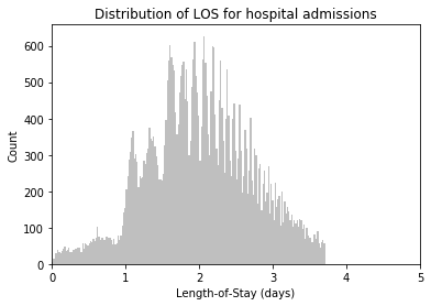
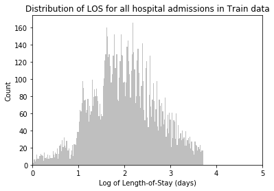
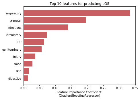
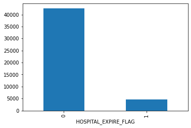
[TOC]
Advanced analytics is transforming all industries and is inherently data hungry. In health care data privacy rules detract data sharing for collaboration. Synthetic data, that retains the original characteristics and model compatible, can make data sharing easy and enable analytics for health care data.
Conventionally statistical methods have been used, but with limited success. Current deidentification techniques are not sufficient to mitigate re-identification risks. Emerging technologies in Deep Learning such as GAN are very promising to solve this problem.
How can you certify that the generated data is as similar and as useful as original data for the intended uses?
The Proposed solution by the team involves generating Synthetic Data using Generative Adversarial Networks or GANs and with the help of conventionally available sources such as TGAN and CTGAN.
The team also wants to build modules which can test the generated synthetic data against the original datasets on following three areas:
- Statistical Similarity: Create standardized modules to check if the generated datasets are similar to the original dataset
- Privacy Risk: Create standardized metrics to check if generated synthetic data protects privacy of all data points in the original dataset.
- Model Compatibility: Compare performance of Machine Learning techniques on original and synthetic datasets
- Statistical Similarity: The generated datasets were similar to each other when compared using PCA and Auto-Encoders.
- Privacy module: The generated Privacy at Risk (PaR) metric and modules helps identify columns which are at risk to expose the privacy of data points from original data. The generated datasets using TGAN and CTGAN had sufficiently high privacy score and protected privacy of original data points.
- Model Compatibility: The synthetic data has comparable model performance for both classification and regression problems.
Optum deals with sensitive healthcare data that has Personal identifiable Information (PII) of 100M+ people and it is expanding every day. The healthcare industry is particularly sensitive as Patient Identifiable Information data is strictly regulated by the Health Insurance Portability and Accountability Act (HIPPA) of 1996. Healthcare firms need to keep customer data secure while leveraging it to innovate research and drive growth in the firm. However, current data sharing practices (to ensure de-identification) have resulted in wait times for data access as long as 3 months. This has proved to be a hindrance to fast innovation at Optum. The need of the hour is to reduce the time for data access and enable innovation while protecting the information of patients. The key question to answer here is:
"How can we safely and efficiently share healthcare data that is useful?"
The key questions involve the inherent trade-off between safety and efficiency. With the inception of big data, efficiency in the data sharing process is of paramount importance. Availability and accessibility of data ensure rapid prototyping and lay down the path for quick innovation in the healthcare industry. Efficient data sharing also unlocks the full potential of analytics and data sciences through use cases like the diagnosis of cancer, predicting response for drug therapy, vaccine developments, drug discovery through bioinformatics. Apart from medical innovation, efficient data sharing helps to bridge the shortcomings in the healthcare system through salesforce effectiveness, managing supply chain and improve patient engagement. While efficient data sharing is crucial, the safety of patient's data can not be ignored. Existing regulations like HIPPA and recent privacy laws like the California Consumer Privacy Act are focused on maintaining the privacy of sensitive information. More advanced attacks are being organized by hackers and criminals aimed at accessing personal information. As per IBM's report on cost data breaches, the cost per record is ~$150. But the goodwill and trust lost by the companies, cannot be quantified So, the balance between data sharing and privacy is tricky.
Existing de-identification techniques involve two main techniques 1) Anonymization Techniques 2) Differential Privacy. Almost every firm relies on these techniques to deal with sensitive information in PII data. These techniques have proven to be successful in the past and thus act as low hanging fruit for any organization.
-
Anonymization techniques: These techniques try to remove the columns which contain sensitive information. Methods include deleting columns, masking elements, quasi-identifiers, k-anonymity, l-diversity, and t-closeness.
-
Differential privacy: This is a perturbation technique which adds noise to columns which introduce randomness to data and thus maintain privacy. It is a mechanism to help to maximize the aggregate utility of databases ensuring high levels of privacy for the participants by striking a balance between utility and privacy.
However, these techniques are not cutting edge when it comes to maintaining privacy and data sharing. Rocher et al have proven that 99.98 percent of Americans (in a sample size of the population of Massachusetts) would be correctly re-identified in any dataset using as few as 15 demographic attributes. They conclude that "even heavily sampled anonymized datasets are unlikely to satisfy the modern standards for anonymization set forth by GDPR and seriously challenge the technical and legal adequacy of the de-identification release-and-forget model.
Proposition
Currently, the field of AI which is being given a lot of importance is Deep Learning. It addresses the critical aspect of data science in this age through universality theorem (identifying function form) and representation learning (correct features). Of late, generative modeling has seen a rise in popularity. In particular, a relatively recent model called Generative Adversarial Networks or GANs introduced by Ian Goodfellow et al. shows promise in producing realistic samples. While this is a state-of-the-art deep learning models to generate new synthetic data, there are few challenges which we need to overcome.
| Salient Features | Challenges |
|---|---|
| Neural Network is cutting edge algorithm in industry | Trained to solve one specific task, can it fit all use cases? |
| Generate image using CNN architecture | Can we generate table from relational databases? |
| Generate fake images of human faces that looks realistic | Would it balance the trade-off between maintaining utility and privacy of data |
| Requires high computational infrastructure like GPUs | How to implement GAN for big data? |
In order to validate the efficacy of GANs to serve our purpose, we propose a methodology for thorough evaluation of synthetic data generated by GANs.
This method is the state of the art in reducing the reidentification risk. As we observed earlier, Data anonymization if effective but reduces the utility, Differential privacy adds small noise but has very bad model compatibility. However, Synthetic data, can be tuned to add privacy without losing either the utility, neither exposing privacy of individual data points. As the data doesn't represent any real entity, the disclosure of sensitive private data is eliminated. If the information available in the released synthetic data matches with any real entity participated in the original data then it is purely a co-incidence which gives individuals plausible deniability
A synthetic dataset is a repository of data that is generated programmatically.
- It can be numerical, binary, or categorical (ordinal or non-ordinal),
- The number of features and length of the dataset should be arbitrary
- It should preferably be random and the user should be able to choose a wide variety of statistical distribution to base this data upon i.e. the underlying random process can be precisely controlled and tuned,
- If it is used for classification algorithms, then the degree of class separation should be controllable to make the learning problem easy or hard
- Random noise can be interjected in a controllable manner
- For a regression problem, a complex, non-linear generative process can be used for sourcing the data
To calculate the similarity between two tables, our methodology transfers the problem into calculating how different the synthetic data generated by GAN algorithm is from the original data. The smaller the difference between two data sets, the more similar they are with each other. In this methodology, the similarity between the synthetic data and original data will be evaluated in two perspectives: the corresponding columns and the relationships between all columns in each tables. The diagram of the metrics is shown below:

Quantifying the difference between two distributions can be referred to calculating the statistical distance between them. However this can be challenging as it can be difficult to interpret the measure. Instead, we can use a more common measurement, Kullback-Leibler Divergence (KL-divergence), to measure the distribution similarity between the pair-columns in both original table and synthetic table. KL-divergence quantifies how much information is lost when we compare the synthetic column distribution with original one. More specifically, the KL-divergence is just a slight modification of our formula for entropy and essentially, in our case, is the expectation of the log difference between the probability of data in the original column distribution(p) with the synthetic column distribution(q). The formula is below:
For the probability distribution of continuous variable:
(A continuous random variable is defined as one which takes an infinite number of possible values.)

For the probability distribution of discrete variable:
(A discrete random variable is defined as one which may take on only a countable number of distinct values and thus can be quantified.)

KL divergence is not symmetric, which means that how different two distributions compared to each other is usually not the same. In this case, KL divergence would be used to calculate how different the synthetic data generated is from the original data. The intuition for KL divergence score is that when the probability for an event from p is large, but the probability for the same event in q is small, then it would result in a large divergence.
KL divergence can be used to measure continuous or discrete probability distributions, but in the latter case the integral of the events is calculated in stead of the sum of the probabilities of the discrete events. It requires the input data to have a sum of 1, it would not be a proper probability distribution otherwise. Therefore, transformation step before calculating the KL divergence is required, which converts the original column-wise data to an array of probability values of different events.
For discrete columns:
Step 1: Convert original data to probability values
Step2: Calculate the Cosine Similarity and KL divergence (if applicable)
Different from how it is for discrete data, it is impossible to generate a specific and accurate probability value for each data points in the sample of continuous data. The probability of continuous data is defined as the area under the pdf curve, so theoretically the probability of each data point is 0. In our use case, the 'length of Stay' is the only continuous variable because both day and the time during the day are considered in this variable. We will round the values of length of stay to make it all integers for better calculating the the similarity of probability distribution. The probability values will be ordered based on the number of length stayed, the number of length stayed that does not show up in the rounded data would be assigned 0 as its probability. For example, if there is no patient staying in the ICU around 6 days, the probability of the value "6" will be assigned as 0.
Even though KL divergence is a good measurement for common cases, it is restricted to be used on two distributions that have the same length of probability distribution. In the case when the generated discrete column has less number of events from the original one, we need to make sure including all events into the probability distribution of the synthetic one by adding 0 as the probability of the omitted event. According to KL-divergence's formula, the probability sequence put in should not contain zero, it would output infinity other wise.
Considering the special property of continuous data, we propose using cosine similarity for calculating the probability list of the continuous data, in order to maintain the closest probability distribution towards the original data.
Cosine similarity is a measure of similarity between two non-zero vectors of an inner product space that measures the cosine of the angle between them. The formula referenced from wiki page is shown below, where A and B in our case is the array of frequency probabilities of each unique value in the synthetic column and original column respectively:
For continuous columns:
**Step 1: **Transform numerical data into values of bins
Step 2: Convert original data to probability values
Step3: Calculate the Cosine Similarity
Limitations:
For some numerical data such as decimal data that ranges only from 0 to 2, it is hard to be rounded up or divided by bins, which will create biases in statistical similarity measurement. In this case, we propose to randomly select the same number of observations as the original data contains for calculating the cosine similarity.
# p and q have to be probability distributions, which means they should be sum of 1.
def kl_divergence(p, q):
    return np.sum(np.where(p != 0, p * np.log(p / q), 0))

from scipy.spatial import distance
def cos_similarity(p,q):
    return 1 - distance.cosine(p, q)
For discrete data:
def discret_probs(column):
    counts = column.value_counts()
    freqs ={counts.index[i]: counts.values[i] for i in range(len(counts.index))}
    probs = []
    for k,v in freqs.items():
        probs.append(v/len(column))
    return np.array(probs)


def cat_plot(colname, realdata, syndata):
    real_p = discret_probs(realdata[colname])
    syn_p = discret_probs(syndata[colname])
    real_plt = pd.DataFrame({colname:realdata[colname], 'table': 'real'})
    syn_plt = pd.DataFrame({colname:realdata[colname], 'table': 'synthetic'})
    df_plt = pd.concat([real_plt, syn_plt], axis=0, sort=False)
    kl = kl_divergence(np.array(real_p), np.array(syn_p))
    cos_sim = cos_similarity(real_p,syn_p)

    plt.figure(figsize = [16, 6])
    plt.title('KL-divergence = %1.3f , Cosine Similarity = %1.3f'% (kl, cos_sim), fontsize = 16)
    sns.countplot(x=colname, hue="table", data=df_plt)
    plt.suptitle('Frequency Distribution Comparison (Column: {})'.format(colname), fontsize = 20)
    plt.xlabel('Categories of Column: {}'.format(colname),fontsize = 14)
    plt.ylabel("Frequency",fontsize = 14)

cat_plot('insurance', real_data, syn_data)
For continuous data:
# identify bin range
max_numlen = max(max(real_data['NUMLABEVENTS']), max(syn_data['NUMLABEVENTS']))
min_numlen = min(min(real_data['NUMLABEVENTS']), min(syn_data['NUMLABEVENTS']))
print('max: ',max_numlen)
print('min: ',min_numlen)
### Decide the bins by yourself:
# The upper bound should be 2 more steps more than the maximum value of both vectors
# Controling the whole length of the bins to around 200 woyld be optimal
bins = np.arange(-50,13800,10)
real_inds = pd.DataFrame(np.digitize(real_data['NUMLABEVENTS'], bins), columns = ['inds'])
syn_inds = pd.DataFrame(np.digitize(syn_data['NUMLABEVENTS'], bins), columns = ['inds'])
from scipy.spatial import distance
def identify_probs(table,column):
counts = table[column].value_counts()
freqs = {counts.index[i]: counts.values[i] for i in range(len(counts.index))}
for i in range(1, len(bins)+1):
if i not in freqs.keys():
freqs[i] = 0
sorted_freqs = {}
for k in sorted(freqs.keys()):
sorted_freqs[k] = freqs[k]
probs = []
for k,v in sorted_freqs.items():
probs.append(v/len(table[column]))
return sorted_freqs, np.array(probs)
real_p = identify_probs(real_inds,'inds')[1]
syn_p = identify_probs(syn_inds,'inds')[1]
def cos_similarity(p,q):
return 1 - distance.cosine(p, q)
cos_sim = cos_similarity(real_p,syn_p)
def num_plot(colname, realdata, syndata):
plt.figure(figsize = [16, 6])
plt.suptitle('Frequency Distribution Comparison (Cosine Similarity: %1.3f )'% cos_sim, fontsize = 18)
plt.subplot(121)
plt.title('Synthetic Data', fontsize = 16)
sns.distplot(syndata[colname], color = 'b', kde = False)
plt.xlabel('Column: {}'.format(colname),fontsize = 14)
plt.ylabel("Frequency",fontsize = 14)
plt.xlim(min(bins), max(bins))
plt.subplot(122)
plt.title('Original Data', fontsize = 16)
sns.distplot(realdata[colname], color = 'r', kde = False)
plt.xlabel('Column: {}'.format(colname) ,fontsize = 14)
plt.ylabel("Frequency",fontsize = 14)
plt.xlim(min(bins), max(bins))
plt.show()
num_plot('NUMLABEVENTS', real_data, syn_data)Dimensionality reduction techniques are proposed to compress high-dimensional table in a way that generates a lower dimensional representation of original table, which further enables similarity score calculation and visualization of the relationships among columns in a table.
Description and Rationale for Autoencoder
Autoencoder is considered as a data compression algorithm and has long been thought to be a potential avenue for solving the problem of unsupervised learning, i.e. the learning of useful representations without the need for labels. Stated from Keras team about Autoencoder, autoencoders are not true unsupervised learning technique (which would imply a different learning process together), they are self-supervised technique, a specific instance of supervised learning where the targets are exactly the input data or generated from the input data.
In our case, the aim of an autoencoder is to learn a representation (embedding) of the relationships among multiple features in our table by setting the input and target data the same. Because Neural Networks can slowly approximate any function that maps inputs to outputs through an iterative optimization process called training. The embedding space has fewer dimensions (columns) than the feature data in a way that captures some latent structure of the feature data set.
Step1: Train an Autoencoder
Autoencoder can be broken in to 2 parts:
- Encoder: this part of the network compresses the input into an assigned number of vectors, which in our case for tabular data is the number of columns. The space represented by these fewer number of vectors is often called the latent-space or bottleneck. These compressed data that represent the original input are together called an “embedding” of the input.
- Decoder: this part of the network tries to reconstruct the input using only the embedding of the input. When the decoder is able to reconstruct the input exactly as it was fed to the encoder, you can say that the encoder is able to produce the best embeddings for the input with which the decoder is able to reconstruct well!
In order to make sure both synthetic table and original table are transformed exactly in the same process, we will train the auto-encoder using the original dataset and then predict on the synthetic dataset using the model built.
Step2: Extracting Embeddings from Autoencoder Network
After training the Autoencoder, extract the embedding for an example from the network. Extract the embedding by using the feature data as input, and read the outputs of the encoder layer. The embedding should contain information about reproducing the original input data, but stored in a compact way.
For the purpose of generating a similarity score, we would assign the dimension of embedding to be 1 so that we can use Cosine similarity or Euclidean distance to calculate the similarity. However, for visualization, we can choose either using autoencoder to compress both tables separately to a lower dimensional (but more than 2) embedding and then use PCA to further compress the data to 2 dimension or using autoencoder to compress both tables directly to 2 dimensional embeddings. In this document, we will demonstrate later with the former method for the purpose of metric diversity.
Step3: Measuring Similarity from Embeddings
Next we would quantify the similarity for pairs of examples by using their embedding vectors.
We now have embeddings for the pair of tables. A similarity measure takes these embeddings and returns a number measuring their similarity. Remember that embeddings are simply vectors of numbers. To find the similarity between two vectors A=[a1,a2,...,an] and B=[b1,b2,...,bn], we can use Cosine Similarity that we mentioned before. It is a better measurement than Euclidean distance because it considers the angle of the vectors by putting them on a high dimensional space for comparison. And it outputs a score that ranges from 0 to 1 where 0 means that two vectors are oriented completely differently and 1 means that two vectors are oriented identically. This makes the comparison of the performances between different GAN algorithms easier.
Because there would be synthetic tables that have a different number of rows than the original table, we would consider the distribution as how we do for column-wise distribution evaluation instead of the pure values of the embeddings. We would take similar steps for
-
The challenge applying Autoencoder with tabular data is the fact that each column represents its unique type of distribution. In other words, data types such as categories, ID numbers, ranks, binary values are all smashed into one sample table.
-
an autoencoder assume that all features (columns) in the table determines the similarity at the same degree, which means that this isn't the optimal choice when certain features could be more important than others in determining similarity.
-
Different settings of bins for calculating the frequency probabilities would result in different cosine similarity scores. The metric for this is not robust enough for an accurate and stable result.
x_train = np.array(x_train)
x_test = np.array(x_test)
# Flatten the data into vectors
x_train = x_train.reshape((len(x_train), np.prod(x_train.shape[1:])))
x_test = x_test.reshape((len(x_test), np.prod(x_test.shape[1:])))
print(x_train.shape)
print(x_test.shape)
from keras.layers import Input, Dense
from keras.models import Model
def modeling_autoencoder(latent_dim, x_train):
original_dim= x_train.shape[1]
# this is our input placeholder
input_data = Input(shape=(original_dim,))
# "encoded" is the encoded representation of the input
encoded = Dense(latent_dim, activation='relu')(input_data)
# "decoded" is the lossy reconstruction of the input
decoded = Dense(original_dim, activation='sigmoid')(encoded)
# this model maps an input to its reconstruction (Define a model that would turn input_data into decoded output)
autoencoder = Model(input_data, decoded)
#### Create a separate encoder model ####
# this model maps an input to its encoded representation
encoder = Model(input_data, encoded)
#### as well as the decoder model ####
# create a placeholder for an encoded (assigned # of dimensions) input
encoded_input = Input(shape=(latent_dim,))
# retrieve the last layer of the autoencoder model
decoder_layer = autoencoder.layers[-1]
# create the decoder model
decoder = Model(encoded_input, decoder_layer(encoded_input))
#### Autoencoder model training ####
autoencoder.compile(optimizer='adadelta', loss='binary_crossentropy')
autoencoder.fit(x_train, x_train,
epochs=50,
batch_size=256,
shuffle=True,
validation_split = 0.2)
return encoder, decoder
trained_encoder = modeling_autoencoder(1, x_train)[0]
encoded_testdata = trained_encoder.predict(x_test)
encoded_traindata = trained_encoder.predict(x_train) Calculate similarity score
### Decide the bins by yourself:
# The upper bound should be 2 more steps more than the maximum value of both vectors

bins = np.arange(0,2100,20)

real_inds = pd.DataFrame(np.digitize(encoded_traindata, bins), columns = ['inds'])
syn_inds = pd.DataFrame(np.digitize(encoded_testdata, bins), columns = ['inds'])

def identify_probs(table,column):
    counts = table[column].value_counts()
    freqs = {counts.index[i]: counts.values[i] for i in range(len(counts.index))}
    for i in range(1, len(bins)+1):
        if i not in freqs.keys():
            freqs[i] = 0
    sorted_freqs = {}
    for k in sorted(freqs.keys()):
        sorted_freqs[k] = freqs[k]
    probs = []
    for k,v in sorted_freqs.items():
        probs.append(v/len(table[column]))
    return sorted_freqs, np.array(probs)

from scipy.spatial import distance

real_p = identify_probs(real_inds,'inds')[1]
syn_p = identify_probs(syn_inds,'inds')[1]
def cos_similarity(p,q):
    return 1 - distance.cosine(p, q)
cos_similarity(real_p,syn_p)For visualization, PCA or t-SNE can be used to generate a lower dimensional data and then visualize them to compare.
Description and Rationale for PCA
Principal Component Analysis (PCA) is a linear feature extraction technique. It performs a linear mapping of the data to a lower-dimensional space in such a way that the variance of the data in the low-dimensional representation is maximized. It does so by calculating the eigenvectors from the covariance matrix. The eigenvectors that correspond to the largest eigenvalues (the principal components) are used to reconstruct a significant fraction of the variance of the original data.
Description and Rationale for t-SNE
t-Distributed Stochastic Neighbor Embedding (t-SNE) is a tool to visualize high-dimensional data. It converts similarities between data points to joint probabilities and tries to minimize the Kullback-Leibler divergence between the joint probabilities of the low-dimensional embedding and the high-dimensional data. However, t-SNE in Scikit learn has a cost function that is not convex according to Scikit learn documentation, which makes two visualizations of two tables generated by the same transformation function not comparable. Because they use different initializations for the transformation, we would get different results.
Therefore, in this document, we would use PCA as techniques for visualization comparison. t-SNE is still a great technique recommended for visualizing high-dimensional data because it is a probabilistic technique compared to PCA that is a mathematical one. Linear dimensionality reduction algorithms, like PCA, concentrate on placing dissimilar data points far apart in a lower dimension representation. But in order to represent high dimension data on low dimension, non-linear manifold, it is essential that similar data points must be represented close together, which is something t-SNE does not PCA.
Step 1: Train autoencoder for a 5-dim embedding using original table, and then predict on synthetic table.
Step 2: Extract the embeddings of original table and synthetic table respectively
Step 3: Train a PCA transformation using the original embedding for reducing the dimension to 2, and use the same transformation for the synthetic embedding.
Step 4: Visualize the results of PCA with two scatter plots
trained_encoder = modeling_autoencoder(5, x_train)[0]
encoded_testdata = trained_encoder.predict(x_test)
encoded_traindata = trained_encoder.predict(x_train)
PCA:
import matplotlib.pyplot as plt
from sklearn.decomposition import PCA

# T-sne visualization
pca = PCA(n_components=2, random_state = 0)
pca_train = pca.fit_transform(encoded_traindata)
pca_test = pca.fit_transform(encoded_testdata)
pca_train_df = pd.DataFrame(data = pca_train, columns = ('Dim_1','Dim_2'))
pca_test_df = pd.DataFrame(data = pca_test, columns = ('Dim_1','Dim_2'))

plt.figure(figsize = [14, 5])
plt.subplot(121)
plt.title('Original dataset')
plt.scatter(pca_train_df['Dim_1'],pca_train_df['Dim_2'], marker = 'o')
plt.xlabel('Dimension 1',fontsize=14)
plt.ylabel('Dimension 2',fontsize=14)
# plt.axis([-1.0, 2.0, -0.5, 1.5])

plt.subplot(122)
plt.title('Synthetic dataset')
plt.scatter(pca_test_df['Dim_1'],pca_test_df['Dim_2'], marker = 'o')
plt.xlabel('Dimension 1',fontsize=14)
plt.ylabel('Dimension 2',fontsize=14)
# plt.axis([-1.0, 2.0, -0.5, 1.5])

plt.show()
t-SNE:
import matplotlib.pyplot as plt
from sklearn.manifold import TSNE

# T-sne visualization
tsne = TSNE(n_components = 2, random_state = 0)
tsne_train = tsne.fit_transform(encoded_traindata)
tsne_test = tsne.fit_transform(encoded_testdata)
tsne_train_df = pd.DataFrame(data = tsne_train, columns = ('Dim_1','Dim_2'))
tsne_test_df = pd.DataFrame(data = tsne_test, columns = ('Dim_1','Dim_2'))

plt.figure(figsize = [14, 5])
plt.subplot(121)
plt.title('Original dataset')
plt.scatter(tsne_train_df['Dim_1'],tsne_train_df['Dim_2'], marker = 'o')
plt.xlabel('Dimension 1',fontsize=14)
plt.ylabel('Dimension 2',fontsize=14)
# plt.axis([-30, 40, -40, 40])

plt.subplot(122)
plt.title('Synthetic dataset')
plt.scatter(tsne_test_df['Dim_1'],tsne_test_df['Dim_2'], marker = 'o')
plt.xlabel('Dimension 1',fontsize=14)
plt.ylabel('Dimension 2',fontsize=14)
# plt.axis([-30, 40, -40, 40])

plt.show()The combination of Autoencoder and dimensionality reduction techniques such as PCA is one way to measure the statistical similarity between two tables. They are done in a self-supervised manner by training the same data as input and output of a special neural network so that it could extract an representation of the input data in a desired dimensional structure. But how are the synthetic data performing in an unsupervised algorithm compared to the original data? Here we will use a unsupervised technique that is classical but widely-used in real business -Clustering - to evaluate the statistical similarity in another perspective.
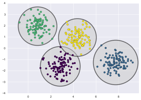
The basic idea of clustering is to organize data objects (which in our case is patients) into homogeneous groups called clusters. The desired properties of clustering result are high intra-similarity (data objects within each cluster) and low inter-similarity (clusters with each other).
We would use the most common approach k-means clustering algorithm for clustering evaluation. Here is k-means idea:
- Choose k data points (objects) at random (They will represent cluster centers, namely means)
- Assign the remaining points to the cluster to which they are most similar (Based on the distance from the cluster mean value)
- Update the means based on newly formed clusters
- Repeat from Step 2 until converges.
Step1: Data Transformation
We use the most popular and widely used distance metric for numeric data, Euclidean Distance, to calculate the distance between data objects. Therefore, we need to convert string values into numerical values using one-hot encoding transformation. Even though one-hot encoding would make it harder to interpret the cluster results because it would keep increasing the space of features, we can use it because we do not need to worry about the interpretation in this case.
Step 2: Define the number of Clusters (Elbow Curve) and clustering modeling
The k-means clustering algorithm requires the number of clusters (k) to be assigned manually. The elbow method is the most common method to validate the number of clusters. The idea of the elbow method is to run k-means clustering on the dataset for a range of values of k, and for each value of k calculate the sum of squared errors (SSE). Then plot a line chart of the SSE for each value of k. If the line chart looks like an arm, then the "elbow" on the arm is the value of k that is the best. The idea is that we want a small SSE, but that the SSE tends to decrease toward 0 as we increase k. So our goal is to choose a small value of k that still has a low SSE, and the elbow usually represents where we start to have diminishing returns by increasing k.
Step 3: Evaluating Clustering result
We will evaluate the similarity of the table by comparing the visualization of the elbow curve and centers of clusters. By comparing the number of clusters indicated by elbow curves and how different centers of different clusters are between the original table and synthetic table, we can get a sense of how similar the features are between data in the original table and the synthetic one.
For Use case 1:
import numpy as np
import pandas as pd
from scipy import stats
from sklearn.cluster import KMeans
import matplotlib.pyplot as plt
import seaborn as sns
from sklearn.preprocessing import StandardScaler

train_tgan=train_tgan.round(0)
train_tgan[train_tgan < 0] = 0

train_ctgan=train_ctgan.round(0)
train_ctgan[train_ctgan < 0] = 0

original=train.iloc[:,1:19]
tgan=train_tgan.iloc[:,1:19]
ctgan=train_ctgan.iloc[:,1:19]

scaler_1 = StandardScaler()
scaler_1.fit(original)
original_scaled=scaler_1.transform(original)

scaler_2 = StandardScaler()
scaler_2.fit(tgan)
tgan_scaled=scaler_2.transform(tgan)

scaler_3 = StandardScaler()
scaler_3.fit(ctgan)
ctgan_scaled=scaler_3.transform(ctgan)

# Original
wcss_original = []
for i in range(1, 20):
    kmeans = KMeans(n_clusters=i, init='k-means++', max_iter=300, n_init=10, random_state=0)
    kmeans.fit(original_scaled)
    wcss_original.append(kmeans.inertia_)

# TGAN
wcss_tgan = []
for i in range(1, 20):
    kmeans = KMeans(n_clusters=i, init='k-means++', max_iter=300, n_init=10, random_state=0)
    kmeans.fit(tgan_scaled)
    wcss_tgan.append(kmeans.inertia_)

# CTGAN
wcss_ctgan = []
for i in range(1, 20):
    kmeans = KMeans(n_clusters=i, init='k-means++', max_iter=300, n_init=10, random_state=0)
    kmeans.fit(ctgan_scaled)
    wcss_ctgan.append(kmeans.inertia_)

# For elbow plots
plt.figure(figsize = [14, 6])
plt.style.use('seaborn')
# Plot 1
plt.subplot(131)
plt.plot(range(1, 20), wcss_original)
plt.title('Elbow Plot (Original Dataset)')
plt.xticks(np.arange(0,20,2))
plt.xlabel('Number of clusters')
plt.ylabel('WCSS')
# Plot 2
plt.subplot(132)
plt.plot(range(1, 20), wcss_tgan)
plt.title('Elbow Plot (TGAN Dataset)')
plt.xticks(np.arange(0,20,2))
plt.xlabel('Number of clusters')
plt.ylabel('WCSS')
# Plot 3
plt.subplot(133)
plt.plot(range(1, 20), wcss_ctgan)
plt.title('Elbow Plot (CTGAN Dataset)')
plt.xticks(np.arange(0,20,2))
plt.xlabel('Number of clusters')
plt.ylabel('WCSS')
# Layout of plots
plt.tight_layout()
plt.show()
Create clusters
kmeans = KMeans(n_clusters=3, init='k-means++', max_iter=300, n_init=10, random_state=0)
kmeans.fit(original_scaled)
original['clusters'] = kmeans.labels_

kmeans = KMeans(n_clusters=3, init='k-means++', max_iter=300, n_init=10, random_state=0)
kmeans.fit(tgan_scaled)
tgan['clusters'] = kmeans.labels_

kmeans = KMeans(n_clusters=3, init='k-means++', max_iter=300, n_init=10, random_state=0)
kmeans.fit(ctgan_scaled)
ctgan['clusters'] = kmeans.labels_

original_means=original.groupby(['clusters']).mean()
tgan_means=tgan.groupby(['clusters']).mean()
ctgan_means=ctgan.groupby(['clusters']).mean()

plt.figure(figsize = [14, 5])
plt.style.use('seaborn')
# Plot 1
plt.subplot(131)
plt.title('Original Data')
plt.scatter(original_means['NUMPROC'],
            original_means['NUMDIAGNOSIS'],
            s=80)
plt.xlim(0,18)
plt.ylim(0,25)
plt.xlabel('NUMPROC')
plt.ylabel('NUMDIAGNOSIS')
# Plot 2
plt.subplot(132)
plt.title('TGAN Data')
plt.scatter(tgan_means['NUMPROC'],
            tgan_means['NUMDIAGNOSIS'],
            s=80)
plt.xlim(0,18)
plt.ylim(0,25)
plt.xlabel('NUMPROC')
plt.ylabel('NUMDIAGNOSIS')
# Plot 3
plt.subplot(133)
plt.title('CTGAN Data')
plt.scatter(ctgan_means['NUMPROC'],
            ctgan_means['NUMDIAGNOSIS'],
            s=80)
plt.xlim(0,18)
plt.ylim(0,25)
plt.xlabel('NUMPROC')
plt.ylabel('NUMDIAGNOSIS')

plt.tight_layout()
plt.show()The synthetic data generated by GAN algorithms can be shared with internal business, academic researchers and third parties to tackle business problems. These stakeholders can then use machine learning algorithms on synthetic data to perform future predictions and create strategies as per their needs. In order to serve these needs, the synthetic data generated should have the same utlity as the original data and provide fairly similar prediction if not exactly same. Thus, it's crucial to evaluate if models generated using synthetic data are compatibile with original data? In this module, we will build different machine learning algorithms on 2 different use cases; a) Length of Stay b) Mortality prediction. The description of use cases can be found under Use cases section. These use cases are selected to evaluate both regression and classification models.
- One hot encoding (optional): In case there are any categorical variables required for prediction, we first need to perform one hot encoding. This is done to make sure we don't miss out any categories in test dataset after splitting data into train and test. Example, in case of ethnicity column, there are multiple types like White, Hispanic, Asian, African etc. If we split data into train and test before performing one hot encoding, then there are chances that no Hispanic is present in test data and only present in train data. This can lead to problems while evaluating accuracy of models.
- Split data into train and test: The analytical data set generated as per the use cases is first split into 2 parts i.e. train and test in the ratio of 80:20. While splitting data set, stratified sampling is performed using the dependent / target variable, duration of stay in use case 1 (length of stay) and expiry flag in use case 2 (mortality prediction).
- Generate Synthetic Data: Train dataset is used as an input to GAN algorithms to generate synthetic data of same name of rows. We generated synthetic data using TGAN and CTGAN which was then used to build models.
- Standarize variables (optional): Numerical variables are present on different scales and some variables cna influence the prediction results more than others. Example, Age and Salary are both numeric variables however, range of salary is much bigger than range of age and thus can impact the prediction results. In order to account for this, we standardized all variables with mean 0 and standard deviation 1. This is same as z-score formula.
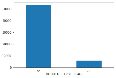
- Model building: Using original train data and synthetic train data (generated by GAN algorithm). For use case 1 (Length of Stay), we used regression algorithms like Regression Tree, Random Forest, XGBoost, Support Vector Machine and K-Nearest Neighbor. For use case 2 (Mortality Prediction), we used classification algrotihms like Logistic Regression, XGBoost and Neural Network. Variety in use cases allows us to evaluate performance of synthetic data on various machine learning algorithms. In classification, due to imbalanced class of target variable, we used parameters within algorithms to assign appropriate weightage to each class.
- Hyperparameter tuning: 5-fold cross validation is performed along with grid search to perform hyperparameter tuning and selected best combination to improve the models. The metrics to evaluate can be different for different use case example, for mortality prediction, focus is on recall because we want to make sure we predict the patients who are going to die and take actions to save lives.
- Prediction: Finally, test data is used for prediction based on models generated and range of metrics were reported to compare performance. For classification, metrics like accuracy, precision, recall, f1-score and AUC-ROC. For regression, metrics like Mean Squared Error, Root Mean Squared Error, Mean Absolute Error, Mean Absolute Percentage Error.
Above image gives us a better idea of the overall process we are going to follow here.
- With the existing data Sources, the team will formulate analytical datasets common use cases with the data such as
- Predicting length of stay in the ICU
- Predicting Hospitality Mortality Rate
- These datasets will be run through various machine learning algorithms ranging from simple, ensemble to Neural networks to evaluate their performance on holdout data to compare their usefulness in real world usage
Along with Statistical similarity and Model compatibility, we need to ensure to minimize reidentification risk for the data points. Current anonymization techniques directly mask user demographics information to protect privacy, but bad actors can still join this data with other databases to identify individuals.
Original data has the best utility but as we mask more and more demographics information for privacy and regulatory reasons, the information provided by the dataset decreases. This in turn slows down research and development which could've potentially saved lives.
Sone of the current industry practices to prevent reidentification include:
Data Anonymization Data anonymization means directly masking the important demographic and personally identifiable attributes from the dataset. Few techniques include:
-
Removal: This process involves removing entire fields of data to reduce the risk of linking it to any source.
-
Redaction: This is used in many forms of government communication. It’s a simple form of removing sensitive information – someone will print out a hard copy of a document and manually mark out sensitive or identifying information before passing it off to another party.
-
Encryption: For the most security, data anonymization isn’t meant to be able to be reversed, but some people and organizations still use encryption as their means of anonymization. Encryption uses technology to render sensitive information as unreadable or unintelligible and can only be read after application of a decryption key, which must be kept separate from the encrypted files. Because there is a decryption key at all, however, there is a higher risk of potentially exposing or accessing sensitive information.
Data breaches have been on the rise, and healthcare firms such as Optum/United Healthcare are particularly vulnerable as they possess extensive Personal Identifiable Information of patients. This significantly hampers the productivity of analysts who need access to datasets, because of long wait times for data access and authorization. Synthetic Data can potentially solve the problem, but there is still a need to compare the privacy risks of synthetic data vs alternatives for businesses to understand the risk involved.
- Reduce the number of columns by removing identifier columns:
Risks: Very common columns like SSN or Patient ID which are unique to a record need to be removed and these definitely reduce the Privacy Risk dramatically as they can be used to join with external tables and mine information. But in practice, these identifier information are not very useful in the use cases for Optum’s research initiatives. The question then becomes - what other columns do we need to drop in order to reduce our Privacy Risk? There is no way to measure which columns make a dataset sensitive.
- Reduce the number of rows:
Risks: We still do not have a quantifiable metric to say how much of Privacy Risk was reduced. The larger risk here is that we arbitrarily remove a fraction of the dataset, this might lead to the dataset becoming less useful. We need to remove rows in a way that retains the usefulness of data, while reducing the risk. Note that every single datapoint that is retained is 100% exposed and can be used by bad actors to mine information (by joining with external tables)
- Synthesize new data that resembles original data
Risks: There is a potential that our synthetic data generation tool presents data that is still relatively close or 100% similar to our original data points if we try to maximize the utility of the dataset too much. We need a metric to still quantify the risk that we accept in these scenarios.
The solution to generate synthetic data has been gaining great traction, but it is still at a nascent stage in terms of research and deployment. A common problem is the idea of coming up with metrics that define the level of privacy achieved in a synthetic dataset, that are easily explainable.
The goal of our methodology document is to define how Optum can define the Privacy Risk in a synthetically created medical dataset. We would like to walk through a new metric/method we developed - ‘Privacy At Risk (PaR)’, how it can be used to define risk in multiple situations, and how PaR values can be used to effectively assess situations and enable quicker data-sharing practices within Optum.
We are predominantly concerned about bad actors being able to join our datasets with the synthetic dataset with outside information to gain access to our PII information. Hence, if there is an opportunity to confuse the bad actor in a way they cannot link a synthetic datapoint to an original datapoint, that is the ideal scenario for us.
We developed the Privacy At Risk Metric based on this opportunity. The PaR Metric works by leveraging the idea of confusion with respect to data records. How many datapoints in our set can be confused for with other people/other records? The higher the confusion, the lesser the chance of a person being re-identified. The focus is primarily on whether including a certain record increases the chance of exposing a person/record and the degree of the exposure.
The Synthetic Data Generation process by itself brings in noise into the data, in a way that maximizes utility while also minimizing the chances of data looking like the original data (hence increasing the confusion aspect)
But there is still a possibility of the synthetic data presenting exact clones of the original datapoints when overfitted while modelling. We need to be able to catch the situations
But what about situations where a synthetic datapoint is x% similar? (x: 0-99). The problem with this approach would mean we need to set thresholds pertaining to every situation. We overcome this problem by bringing the problem down to a relative scale within the dataset, by comparing External and Internal Similarity to assess the level of confusion as a binary variable.
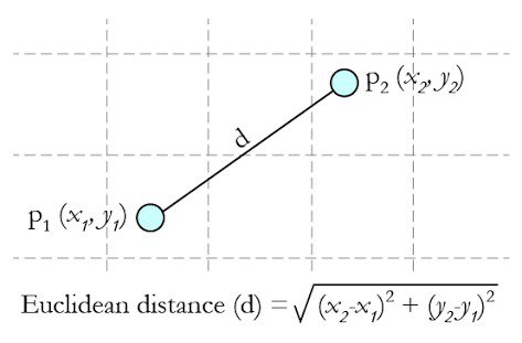
For every datapoint in the original dataset, we would like to see how similar datapoints in the synthetic dataset are using distance/similarity metrics. For our analysis, we primarily use Euclidean distance after one-hot encoding.
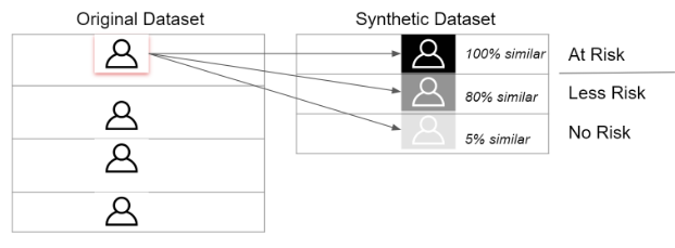
For every data point in the Original Dataset, we need to look at what records in the synthetic dataset are the most similar. This is the idea of ‘External Similarity’.
Let’s say for Person A in Original Dataset: Record 1 in synthetic dataset is 100% similar. This means that our synthetic data generation process has been practically useless for this user’s privacy. The bad actor can still completely leverage the information in the synthetic data to find this user and mine information.
from IPython.display import Image
Image(filename='external_d.png')
But we can observe Record 3 is only 5% similar, the chances of a bad actor using Record 3 to find Person A is extremely low.
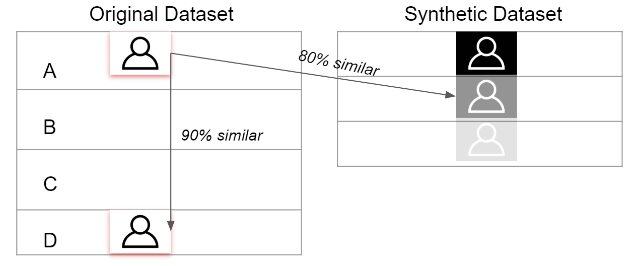
But let’s now look at Record 3. We have an 80% similarity. Intuitively we may think this record is risky for us. But how do we draw a threshold to say what constitutes a risky data point and not? Is it really a risky data point, rather?
In this example you can see that although Person A is 80% similar with Record 2; We can also note that Person A is 90% similar to Person D. This is the idea of ‘Internal Similarity’
What this essentially means is there is a higher chance of connecting Person A with Person B rather than connecting Person A with the synthetic Record 3.
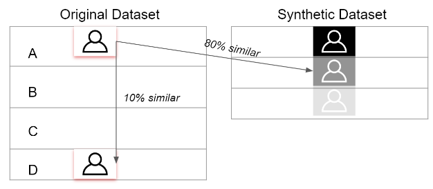
Let’s now look at the counter-scenario
Now we can see the closest resemblance to A inside the Original Dataset is D again, but they are only 10% similar. So that means Person A is already a stand-out unique record. On top of this, our Synthetic Dataset Record 2 is now 80% similar. So when a bad actor gets access to Record 2, there is a high chance they can connect it with Person A and nobody else without any confusion. We need to avoid these scenarios.
Summarizing,
-
Internal Similarity > External Similarity : Ideal Data Point for us; Bad actors cannot attribute a data point to a single person/original record.
-
External Similarity > Internal Similarity: Risky Data Point for us; The record in synthetic dataset is so unique that the synthetic data record can only point to one user record and hence increases the privacy risk of that data point.
-
Hence Privacy Risk = Number of Risky Points / (Number of Ideal Points + Number of Risky Points)
PaR is a conservative metric
A Privacy at Risk value of 6% does not mean 6% of the records are exposed to bad actors. It only means that there is a higher potential of a bad actor trying to interpret the synthetic information to a real record/person with 6% of the records. The inherent assumption here is that all the records in the original dataset are potentially vulnerable.
Determining which synthetic data records are similar to the original dataset
In this case, one record constitutes a single real person (as in our examples) and one person has only one record in the table.
We use our synthetic data generation techniques to come up with an equal number of 'fake' people for the synthetic dataset.
So the question becomes : Which of the fake people's information can be used to connect back to the original person and mine their information? Hence we need to find out how similar are original person information these fake people.
We compute similarity using Distance Metrics in this analysis.
There are a number of Distance Metrics to choose from - Euclidean, Manhattan, Gower Distance (which can handle categorical and continuous variables) and so on.
Column Matches as Similarity Metric
This can be used as an extremely conservative metric where we only look for exact matches between columns of Synthetic Data and Original Data. This can help us spot exact matches between Original Data and Synthetic Data more efficiently. It can be used in situations where the use case mandates we only worry about privacy risk in situations that are an exact match and can hence be traced back.
But for this analysis, we prefer to use the simple Euclidean distance after one-hot encoding the data.
A lower value of Euclidean Distance means a higher degree of similarity and vice versa.
We go about computing the distance between every single datapoint in the Original Dataset with every other point in the Synthetic Dataset.
These are all the External Distances we obtain as a matrix of size: Length of Original Dataset x Length of Synthetic Dataset
We also need to compute the Internal Distances so that we can compare the External Distance vs Internal Distance for every real Person in the dataset.
Internal Distances matrix of size: Length of Original Dataset x Length of Original Dataset
A note: Normalization is extremely important here
We only wish to look at the closest/most similar records given a real person in the Original Dataset. The way bad actors can obtain information about this real person is by leveraging a very similar looking record and connect it to a real person's information outside.
But defining 'close' is subjective. A simple approach would be to use n=1 ie. only look at the closest person in the synthetic dataset (External Similarity), and the closest other person in the original dataset (Internal Similarity)
There's always an option to extend this into a radius of close people. By setting n=5, we can always look at the closest 5 people in Original and Synthetic datasets to achieve an idea of how close are records on average.
Distance metrics, by default, may not account for domain knowledge about what defines similarity. Hence, a weighted distance metric might yield bette results for a defined problem, given domain knowledge.
In our scenario, we are dealing with Mortality information of Patients in ICU Wards. We know that information like Gender, Ethnicity and Age can often be used to join with External Datasets and mine patient's personally identifiable information.
Hence, we might modify the Euclidean Distance to add a lower weight for features of Gender, Age and Ethnicity. When we add lower weights for highly sensitive fields, we report higher similarity and we will be better able to catch risky situations often.
This case will be dealt with differently with respect to Internal Similarity.
In this scenario, when we compare a single record with every other record in the same Original Dataset - we are not really answering the question of whether there is another person who really resembles this person/record. The problem here is each person might have multiple records. Hence when we compute Internal Similarity, we may end up finding 'similar people' always when those are all records belonging to the same person.
Hence the solution is to only look at records belonging to other users / patients in our use case. We use the Patient ID information to determine which records belong to which user. Hence:
Internal Similarity is the distance of a given datapoint to every other datapoint belonging to a different user.
The PaR module is more driven on a broad concept and hence can be extremely tailored and used for different situations.
-
Column Subset Analysis - Often bad actors may have access to only 3 or 4 fields about a certain person whose information they wish to mine. The way they would go about re-identifying these individuals is by querying for these attributes and finding the closest match. More broadly, the business could only be concerned about a few columns that are highly sensitive to the business. We can filter for only these columns and estimate Privacy at Risk values.
-
Choice of distance metric is driven by the level of privacy needed for the use case. The way we compute similarity can be simply changed by the choice of function - be it Euclidean, Gower Distance or Cosine Similarity or Exact Matching
-
Feature Weighting In cases we know the sensitivity of features, we can specify the way we measure similarity by assigning weights to the features we pass into the Privacy Risk Estimator. This allows for a more tailored estimate of the risk associated with the synthetic dataset.
-
Ability to handle different types of datasets With the module, we can handle both Personal Information scenarios, eg: Member Data and Journey scenarios eg: Claims data. The idea of individuals within the Privacy Risk calculations can be extended to entities as well - the question becomes 'Will an entity be exposed given the synthetic data?'
A generative adversarial network (GAN) is a class of machine learning systems invented by Ian Goodfellow in 2014. GAN uses algorithmic architectures that use two neural networks, pitting one against the other (thus the “adversarial”) in order to generate new, synthetic instances of data that can pass for real data.
GANs consist of Two neural networks contest with each other in a game. Given a training set, this technique learns to generate new data with the same statistics as the training set. The two Neural Networks are named Generator and a Discriminator.
Generator The generator is a neural network that models a transform function. It takes as input a simple random variable and must return, once trained, a random variable that follows the targeted distribution. The generator randomly feeds actual image and generated images to the Discriminator. The generator starts with Generating random noise and changes its outputs as per the Discriminator. If the Discriminator is successfully able to identify that generate input is fake, then then its weights are adjusted to reduce the error.
Discriminator The Discriminators job is to determine if the data fed by the generator is real or fake. The discriminator is first trained on real data, so that it can identify it to acceptable accuracy. If the Discriminator is not trained properly, then it in turn will not be accurately able to identify fake images thus poorly training the Generator.
This is continued for multiple iterations till the discriminator can identify the real/fake images purely by chance only.
-
Algorithm: Now lets see how GANs algorithm works internally.
-
- The generator randomly feeds real data mixed with generated fake data for the discriminator
- To begin, in first few iterations, the generator produces random noise which the discriminator is very good at detecting that the produced image is fake.
- Every iteration, the discriminator catches a generated image as fake, the generator readjusts its weights to improve itself. much like the Gradient Descent algorithm
- Over time, after multiple iterations, the generator becomes very good at producing images which can now fool the discriminator and pass as real ones.
- Now, its discriminators turn to improve its detection algorithm by adjusting its network weights.
- This game continues till a point where the discriminator is unable to distinguish a real image from fake and can only guess by chance.
This methodology has been created from the work provided in this paper:
Synthesizing Tabular Data using Generative Adversarial Networks
and this python package
https://pypi.org/project/tgan/
Generative adversarial networks (GANs) implicitly learn the probability distribution of a dataset and can draw samples from the distribution. Tabular GAN (TGAN) is a a generative adversarial network which can generate tabular databy learning distribution of the existing training datasets and can generate samples which are . Using the power of deep neural networks.
TGAN focuses on generating tabular data with mixed variable types (multinomial/discrete and continuous) and propose TGAN. To achieve this, we use LSTM with attention in order to generate data column by column. To asses, we first statistically evaluate the synthetic data generated by TGAN.
The paper also evaluates Machine learning models performance against traditional methods like modelling a multivariate probability or randomization based models.
For a table containing discrete and continuous random variables, They follow some probability distribution. Each row in the table is a sample from this distribution, whihch is sampled independently and the algorithms learn a generative model such that samples generated from this model can satisfy two conditions:
- A Machine Learning model using the Synthetic table achieves similar accuracy on the test table
- Mutual information between an arbitrary pait of variables is similar
Numerical Variables
For the model to learn the data effectively, a reversible transformation is applied. The a numerical variables are converted into a scalar in the range (1, 1) and a multinomial distribution, and convert a discrete variable into a multinomial distribution.
Often, numerical variables in tabular datasets follows multimodal distribution. Gaussian Kernal density estimation is used to estimate these number of noes in the continuous variable. To sample values from these, a gaussian mixture model is used.
Categorical Variables - Improvement needed
categorical variables are directly converted to to one-hot-encoding representation and add noise to binary variables
In TGAN, the the discriminator D tries to distinguish whether the data is from the real distribution, while the generator G generates synthetic data and tries to fool the discriminator. the algorithm uses a Long Short Term Memory(LSTM) as generator and a Multi Layer Perceptron (MLP) as a discriminator.
import warnings
warnings.filterwarnings('ignore')

import pandas as pd
import tensorflow as tf
from tgan.model import TGANModel
from tgan.data import load_demo_data
def tgan_run(data, cont_columns):
tgan = TGANModel(continuous_columns)
return tgan.fit(data)
def tgan_samples(model, num_samples):
return tgan.sample(100000)CTGAN is a GAN-based method to model tabular data distribution and sample rows from the distribution. CTGAN implements mode-specific normalization to overcome the non-Gaussian and multimodal distribution (Section 4.2). We design a conditional generator and training-by-sampling to deal with the imbalanced discrete columns (Section 4.3). And we use fully-connected networks and several recent techniques to train a high-quality model.
Several unique properties of tabular data challenge the design of a GAN model.
- Mixed data types Real-world tabular data consists of mixed types. To simultaneously generate a mix of discrete and continuous columns, GANs must apply both softmax and tanh on the output.
- Non-Gaussian distributions: In images, pixels’ values follow a Gaussian-like distribution, which can be normalized to [−1, 1] using a min-max transformation. A tanh function is usually employed in the last layer of a network to output a value in this range. Continuous values in tabular data are usually non-Gaussian where min-max transformation will lead to vanishing gradient problem.
- Multimodal distributions. We use kernel density estimation to estimate the number of modes in a column. We observe that 57/123 continuous columns in our 8 real-world datasets have multiple modes. Srivastava et al. [21] showed that vanilla GAN couldn’t model all modes on a simple 2D dataset; thus it would also struggle in modeling the multimodal distribution of continuous columns.
- Learning from sparse one-hot-encoded vectors. When generating synthetic samples, a generative model is trained to generate a probability distribution over all categories using softmax, while the real data is represented in one-hot vector. This is problematic because a trivial discriminator can simply distinguish real and fake data by checking the distribution’s sparseness instead of considering the overall realness of a row.
- Highly imbalanced categorical columns. In our datasets we noticed that 636/1048 of the categorical columns are highly imbalanced, in which the major category appears in more than 90% of the rows. This creates severe mode collapse. Missing a minor category only causes tiny changes to the data distribution that is hard to be detected by the discriminator. Imbalanced data also leads to insufficient training opportunities for minor classes.
When feeding data to the GAN algorithm, CTGAN samples so that all categories are correctly represented. Specifically, the goal is to resample efficiently in a way that all the categories from discrete attributes are sampled evenly (but not necessary uniformly) during the training process, and to recover the (not-resampled) real data distribution during test
These three things need to be incorporated:
- Modify the input for conditional vector creation
- The generated rows should preserve the condition
- The conditional generator should learn the real data conditional distribution
import pandas as pd
import tensorflow as tf

from ctgan import load_demo
from ctgan import CTGANSynthesizer
data = load_demo()
discrete_columns = ['workclass','education', 'marital-status', 'occupation', 'relationship', 'race', 'sex','native-country', 'income']
ctgan = CTGANSynthesizer()
ctgan.fit(data, discrete_columns)Source: https://arxiv.org/pdf/1802.06739.pdf
One common issue in above proposed methodologies in GANs is that the density of the learned generative distribution could concentrate on the training data points, meaning that they can easily remember training samples due to the high model complexity of deep networks. This becomes a major concern when GANs are applied to private or sensitive data such as patient medical records, and the concentration of distribution may divulge critical patient information. Differentially Private GANs is achieved by adding carefully designed noise to gradients during the learning procedure.
DPGAN focuses on preserving the privacy during the training procedure instead of adding noise on the final parameters directly, which usually suffers from low utility. Noise is added to the gradient of the Wasserstein distance with respect to the training data.
Note: Wasserstein distance is a distance function defined between probability distributions on a given metric space
The algorithm guarantees that the parameters of discriminator and generator have differential privacy with respect to the sample training points. The algorithm inputs noise e in the generator parameters which enables this privacy, however one needs to perform a grid search over a large range of noise parameter e to get best results.
Source: https://arxiv.org/pdf/1906.09338.pdf
Generative Adversarial Networks (GAN) provide a powerful method for using real data to generate synthetic data but it does not provide any rigorous privacy guarantees. PATE GAN modifies the existing GAN algorithm in a way that does guarantee privacy
PATE GAN consists of two generator blocks called student block and teacher block on top of the existing generator block. With traditional privacy techniques, it is possible for the Generator to reconstruct the original data even after adding noise. PATE GAN prevents this by breaking down the generator into three stages. After the generator creates the data and adds noise, there is an ensemble block which factors in majority voting to create the input. After this there is a student block which aggregates the inputs from the teacher blocks and generates the final data.
The synthetic data is (differentially) private with respect to the original data DP-GAN: The key idea is that noise is added to the gradient of the discriminator during training to create differential privacy guarantees. Our method is similar in spirit; during training of the discriminator differentially private training data is used, which results in noisy gradients, however, we use the mechanism introduced in A noticeable difference is that the adversarial training is no longer symmetrical: the teachers are now being trained to improve their loss with respect to G but G is being trained to improve its loss with respect to the student S which in turn is being trained to improve its loss with respect to the teachers.
Theoretically, the generator in GAN has the potential of generating an universal distribution, which is a superset of the real distribution, so it is not necessary for the student discriminator to be trained on real records. However, such a theoretical bound is loose. In practice, if a generator does generate enough samples from the universal distribution, there would be a convergence issue. On the other hand, when the generator does converge, it no longer covers the universal distribution, so the student generator may fail to learn the real distribution without seeing real records.
It is not necessary to ensure differential privacy for the discriminator in order to train a differentially private generator. As long as we ensure differential privacy on the information flow from the discriminator to the generator, it is sufficient to guarantee the privacy property for the generator. Therefore, instead of focusing on ensuring differential privacy for the whole GAN framework, we design a novel framework to guarantee that all information flowed from the discriminator to the generator satisfies differential privacy.
Compared to PATE-GAN, our approach has two advantages. First, we improve the use of privacy budget by applying it to the part of the model that actually needs to be released for data generation. Second, our discriminator can be trained on real data because itself does not need to satisfy differential privacy. The teacher discriminators do not need to be published, so they can be trained with non-private algorithms.
In addition, we design a gradient aggregator to collect information from teacher discriminators and combine them in a differentially private fashion. Unlike PATE-GAN, G-PATE does not require any student discriminator. The teacher discriminators are directly connected to the student generator. The gradient aggregator sanitizes the information flow from the teacher discriminators to the student generator to ensure differential privacy The privacy property is achieved by sanitizing all information propagated from the discriminators to the generator.
We used MIMIC-III data for this project as it is an open source dataset and contains multiple tables which can be combined to prepare use cases. Data can be accesed on link provided below and in order to access data, few certifications are required which can be obtained by completing trainings on website. Medical Information Mart for Intensive Care Unit (MIMIC) III: Open source dataset developed by the MIT Lab comprising de-identified health data is a comprehensive clinical dataset of 40,000+ patients admitted in ICU. Few salient features of this databases include:
- 26 tables: Comprehensive clinical dataset with different tables
- 40,000+ patients: Data associated with multiple admissions of patients
- 65,000+ ICU admissions: Admitted in ICUs at Beth Israel Deaconess Medical Centre, Boston, from 2001 to 2012
- PII data: Includes patient sensitive details like demographics, diagnosis, laboratory tests, medications etc.
- Use cases: Can be used for multiple analysis like clinical data (prescriptions), claims data (payer), members data (patient)
For this project, we focus on using specific tables from this database and create 2 different use cases which can be found in following section.
Source: https://mimic.physionet.org/gettingstarted/overview/
Predicting the length of stay in ICU using 4 out of 26 tables
Use case: Out of variety of possible use cases from MIMIC III dataset we focus on single use case to predict the number of days a patient stays in the ICU to further generate synthetic data. This usecase seemed important to us because its always a benefit for payer to predict the tendency of the length of stay of a patient. It helps in changing the premium charged by the payer according to the comparison of predictions and baseline (the defined no. of days covered by a particular plan of the patient). For this use case the model utilises the total number of diagnosis that occured for different disease category for each patient.
To build this use case we focus on primarily 4 tables.
- Patients: Every unique patient in the database (defines SUBJECT_ID) Columns like: SUBJECT_ID, GENDER (count of rows: 46520 count of columns: 7)
- Admissions: Every unique hospitalization for each patient in the database (defines HADM_ID) Columns like: SUBJECT_ID, HADM_ID, HOSPITAL_EXPIRE_FLAG, MARITAL_STATUS, ETHNICITY, ADMISSION_TYPE (count of rows: 58976 count of columns: 18 )
- ICUSTAYS: Every unique ICU stay in the database (defines ICUSTAY_ID) Columns like: SUBJECT_ID, HADM_ID, LOS (count of rows: 61532 count of columns: 11 )
- Diagnosis_ICD: Hospital assigned diagnoses, coded using the International Statistical Classification of Diseases and Related Health Problems (ICD) system Columns like: SUBJECT_ID, HADM_ID, NUMDIAGNOSIS (count of rows: 651047 count of columns: 5)
- Load csv files: Read the comma seperated files donwloaded from link (https://mimic.physionet.org/gettingstarted/overview/)
- Merge tables: Use 'SUBJECT_ID' to merge tables like ADMISSIONS, PATIENTS and ICU_STAYS and finally concatenate 'SUBJECT_ID' and 'HADM_ID' to form 'final_id' as composite key.
- Prepare diagnosis dataset: DIAGNOSIS_ICD table is used to map the disease category type using the first three code digits if ICD-9 code. The mapping is used to convert the unique 6984 ICD-9 codes into 18 different disease area categories and finally concatenate 'SUBJECT_ID' and 'HADM_ID' to form 'final_id' as composite key..
- Pivot up diagnosis dataset: After the mapping the disease categories using ICD-9 codes, the datset is pivoted up at the level of the 18 disease categories and the total count of diagnosis is being populated across 'final_id'
- Merge pivoted diagnosis datset to the main dataset: Finally, the above generated dataset is then merged to the main dataset using the 'final_id' as the key.
Note: 6984 ICD-9 codes: The diagnosis dataset contains unique International Classification of Disease (ICD-9) codes 18 primary categories: We consider categories of conditions for the predictive modeling Finally only the relevant columns required for the analysis are selected and we use the dataset for the synthetic data generation. The final data has 116354 rows and 27 columns.
-
Level of data: Each instance in the final data set is unique admission for each patient and is defined by concatination of 'SUBJECT_ID' and 'HADM_ID' to form 'final_id'
-
Target Variables: 'LOS' (length of stay) is used as target variable
-
Predictor variables: 18 columns of different diagnosis category are used as predictor varibales. These 18 categories are: "certain conditions originating in the perinatal period" "complications of pregnancy, childbirth, and the puerperium", "congenital anomalies", "diseases of the blood and blood-forming organs", "diseases of the circulatory system", "diseases of the digestive system", "diseases of the genitourinary system", "diseases of the musculoskeletal system and connective tissue", "diseases of the nervous system", "diseases of the respiratory system", "diseases of the sense organs", "diseases of the skin and subcutaneous tissue", "endocrine, nutritional and metabolic diseases, and immunity disorders", "external causes of injury and supplemental classification", "infectious and parasitic diseases", "injury and poisoning", "mental disorders", "neoplasms" and "symptoms, signs, and ill-defined conditions".
-
Other descriptive variables:
"ADMISSION_TYPE", "INSURANCE", "ETHNICITY", "HOSPITAL_EXPIRE_FLAG", "GENDER" and "EXPIRE_FLAG"
Code (data wrangling performed in R)
- Import required libraries and read csv files
- Function for data preparation
1. Import required libraries and read csv files
install.packages('reshape')
library(reshape2)
library(dplyr)
2. Function for data preparation
# Note this code was written in R
# This code uses the filenames of admission, patients, icustays and diagnosis dataset as the input to the function usecase_1


usecase_1 <- function(admissions,patients,icustays,diagnosis)
{

    #################### Loading datasets ##############################################

    adm <-read.csv(admissions)
    pat <- read.csv(patients)
    icu <- read.csv(icustays)
    diagn <- read.csv(diagnosis)
    map <- read.csv("mapping.csv")

    #################### Selecting specifc columns #####################################

    adm <- adm[,2:ncol(adm)]
    pat <- pat[,2:ncol(pat)]
    icu <- icu[,2:ncol(icu)]
    pres <- pres[,2:ncol(pres)]

    #################### Merging various tables ########################################

    merged_1<- merge(x=adm,y=pat,by.x = c("SUBJECT_ID"), by.y=c("SUBJECT_ID"))
    merged_2<- merge(x=merged_1,y=icu,by.x = c("SUBJECT_ID"), by.y=c("SUBJECT_ID"))

    #################### Data wrangling on Diagnosis dataset ###########################

    diagnosis_unique <- data.frame(unique(diagn$ICD9_CODE)
    names(diagnosis_unique)[1] <-"icd9"
    merged_diag<- merge(x=diagnosis_unique,y=map,by.x = c("icd9"), by.y=c("icd"))
    final_map <- merged_diag[,c(1,4)]
    diagn_final <- merge(x=final_map,y=diagn,by.x = c("icd9"), by.y=c("ICD9_CODE"))
    diagn_final$final_id <-paste(diagn_final$SUBJECT_ID,diagn_final$HADM_ID, sep="_")
    diagn_final$count <-1
    diagn_final <- diagn_final[,c(2,7,8)]

    #################### Pivoting up Diagnosis dataset #################################

    step1<- dcast(data = diagn_final, formula = final_id ~ icd_chp, fun.aggregate = sum, value.var = "count")
    merged_2$final_id <-paste(merged_2$SUBJECT_ID,merged_2$HADM_ID.x, sep="_")

    #################### Merging pivotted up diagnosis dataset with main dataset #######

    merged_3<- merge(x=merged_2,y=step1,by.x = c("final_id"), by.y=c("final_id"))
    merged_3 <- merged_3[,c(1,7,10,14,18,20,25,35,36:54)]
    merged_3 <- merged_3%>%filter(LOS!="NA")
}

# Finally write the database to be used as an input for various GAN algorithms
write.csv(merged_3,"full_database_los_v1.csv")Another use case which we implemented using MIMIC-III dataset is for mortality prediction. This use case is inspired by Kaggle kernel (reference below) where one can predict mortality just by the number of interactions betweeen patient and hospital as predictors through count of lab tests, prescriptions, and procedures. It can be used to evaluate privacy risk with the help of PII columns like GENDER, ETHNICITY, MARITAL_STATUS and also serves as classification problem where we have to predict if patient will expire or not for a single hospital admission.
Reference: https://www.kaggle.com/drscarlat/predict-hospital-mortality-mimic3
Tables Used
- Patients - Every unique patient in the database (defines SUBJECT_ID) Columns like: SUBJECT_ID, GENDER
- Admissions - Every unique hospitalization for each patient in the database (defines HADM_ID) Columns Like: SUBJECT_ID, HADM_ID, HOSPITAL_EXPIRE_FLAG, MARITAL_STATUS, ETHNICITY, ADMISSION_TYPE
- CallOut - Information regarding when a patient was cleared for ICU discharge and when the patient was actually discharged Columns Like: SUBJECT_ID, HADM_ID, NUMCALLOUT (count of rows)
- CPTEvents - Procedures recorded as Current Procedural Terminology (CPT) codes Columns Like: SUBJECT_ID, HADM_ID, NUMCPTEVENTS (count of rows)
- Diagnosis_ICD - Hospital assigned diagnoses, coded using the International Statistical Classification of Diseases and Related Health Problems (ICD) system Columns Like: SUBJECT_ID, HADM_ID, NUMDIAGNOSIS (count of rows)
- Inputevents_CV - Intake for patients monitored using the Philips CareVue system while in the ICU Columns Like: SUBJECT_ID, HADM_ID, NUMINPUTEVENTS (count of rows)
- Labevents - Laboratory measurements for patients both within the hospital and in out patient clinics Columns Like: SUBJECT_ID, HADM_ID, NUMLABEVENTS (count of rows)
- Noteevents - Deidentified notes, including nursing and physician notes, ECG reports, imaging reports, and discharge summaries. Columns Like: SUBJECT_ID, HADM_ID, NUMNOTEVENTS (count of rows)
- Outputevents - Output information for patients while in the ICU Columns Like: SUBJECT_ID, HADM_ID, NUMOUTEVENTS (count of rows)
- Prescriptions - Medications ordered, and not necessarily administered, for a given patient Columns Like: SUBJECT_ID, HADM_ID, NUMRX (count of rows)
- Procedureevents_mv - Patient procedures for the subset of patients who were monitored in the ICU using the iMDSoft MetaVision system. Columns Like: SUBJECT_ID, HADM_ID, NUMPROCEVENTS (count of rows)
- MICROBIOLOGYEVENTS - Microbiology measurements and sensitivities from the hospital database Columns Like: SUBJECT_ID, HADM_ID, NUMMICROLABEVENTS (count of rows)
- Procedures_icd - Patient procedures, coded using the International Statistical Classification of Diseases and Related Health Problems (ICD) system Columns Like: SUBJECT_ID, HADM_ID, NUMPROC (count of rows)
- Transfers - Patient movement from bed to bed within the hospital, including ICU admission and discharge Columns Like: SUBJECT_ID, HADM_ID, NUMTRANSFERS (count of rows)
Final data includes
- Level of data: Each instance in the final data set is one admission and is defined by 'SUBJECT_ID', 'HADM_ID'
- Target Variables: 'HOSPITAL_EXPIRY_FLAG' is used as target variable
- Predictor variables: 'ADMISSION_TYPE', 'MARITAL_STATUS', 'ETHNICITY', 'HOSPITAL_EXPIRE_FLAG', 'GENDER', 'NUMCALLOUT', 'NUMCPTEVENTS', 'NUMDIAGNOSIS', 'NUMOUTEVENTS', 'NUMRX', 'NUMPROCEVENTS', 'NUMMICROLABEVENTS', 'NUMPROC', 'NUMTRANSFERS', 'NUMINPUTEVENTS', 'NUMLABEVENTS', 'NUMNOTEVENTS'
Methodology
- Load csv files: Read the comma separated files downloaded from link (https://mimic.physionet.org/gettingstarted/overview/)
- Roll up tables: We need count of various events or interactions between patients and hospital. In order to do this, group by or aggregate the tables at 'SUBJECT_ID' and 'HADM_ID' level and take count of number of rows for each. This will give total count of events related to single hospital admission.
- Merge tables: Use 'SUBJECT_ID' and 'HADM_ID' as composite key to merge all tables together and create final analytical data set.
Code
- Import required libraries and read csv files
- Function to roll up tables
- Merge all tables
- Exploratory Analysis
Import required libraries and read csv files
import pandas as pd
import matplotlib.pyplot as plt
from sklearn.model_selection import train_test_split
import warnings
warnings.filterwarnings('ignore')
patients = pd.read_csv("data/patients.csv")
admissions = pd.read_csv("data/admissions.csv")
callout = pd.read_csv("data/callout.csv")
cptevents = pd.read_csv("data/cptevents.csv")
diagnosis = pd.read_csv("data/diagnoses_icd.csv")
outputevents = pd.read_csv("data/outputevents.csv")
rx = pd.read_csv("data/prescriptions.csv")
procevents = pd.read_csv("data/procedureevents_mv.csv")
microlabevents = pd.read_csv("data/microbiologyevents.csv")
proc = pd.read_csv("data/procedures_icd.csv")
transfers = pd.read_csv("data/transfers.csv")
inputevents = pd.read_csv("data/inputevents_cv.csv")
labevents = pd.read_csv("data/labevents.csv")
noteevents = pd.read_csv("data/noteevents.csv")Function to roll up tables
def rollup_sub_adm(df,col):
    df=df.groupby(['SUBJECT_ID','HADM_ID']).agg({'ROW_ID':'count'})
    df.reset_index(inplace=True)
    df.columns=['SUBJECT_ID','HADM_ID',col]
    print(col,":",df.shape)
return dfcallout=rollup_sub_adm(callout,'NUMCALLOUT')
cptevents=rollup_sub_adm(cptevents,'NUMCPTEVENTS')
diagnosis=rollup_sub_adm(diagnosis,'NUMDIAGNOSIS')
outputevents=rollup_sub_adm(outputevents,'NUMOUTEVENTS')
rx=rollup_sub_adm(rx,'NUMRX')
procevents=rollup_sub_adm(procevents,'NUMPROCEVENTS')
microlabevents=rollup_sub_adm(microlabevents,'NUMMICROLABEVENTS')
proc=rollup_sub_adm(proc,'NUMPROC')
transfers=rollup_sub_adm(transfers,'NUMTRANSFERS')
inputevents=rollup_sub_adm(inputevents,'NUMINPUTEVENTS')
labevents=rollup_sub_adm(labevents,'NUMLABEVENTS')
noteevents=rollup_sub_adm(noteevents,'NUMNOTEVENTS')NUMCALLOUT : (28732, 3)
NUMCPTEVENTS : (44148, 3)
NUMDIAGNOSIS : (58976, 3)
NUMOUTEVENTS : (52008, 3)
NUMRX : (50216, 3)
NUMPROCEVENTS : (21894, 3)
NUMMICROLABEVENTS : (48740, 3)
NUMPROC : (52243, 3)
NUMTRANSFERS : (58976, 3)
NUMINPUTEVENTS : (31970, 3)
NUMLABEVENTS : (58151, 3)
NUMNOTEVENTS : (58361, 3)
Merge all tables
mortality=admissions[['SUBJECT_ID','HADM_ID','ADMISSION_TYPE','MARITAL_STATUS','ETHNICITY','HOSPITAL_EXPIRE_FLAG']]
mortality.loc[pd.isnull(mortality['MARITAL_STATUS']),'MARITAL_STATUS'] ='UNKNOWN (DEFAULT)'
mortality = mortality.merge(patients[['SUBJECT_ID','GENDER']],how='left',on='SUBJECT_ID')
mortality = mortality.merge(callout,how='left',on=['SUBJECT_ID','HADM_ID'])
mortality = mortality.merge(cptevents,how='left',on=['SUBJECT_ID','HADM_ID'])
mortality = mortality.merge(diagnosis,how='left',on=['SUBJECT_ID','HADM_ID'])
mortality = mortality.merge(outputevents,how='left',on=['SUBJECT_ID','HADM_ID'])
mortality = mortality.merge(rx,how='left',on=['SUBJECT_ID','HADM_ID'])
mortality = mortality.merge(procevents,how='left',on=['SUBJECT_ID','HADM_ID'])
mortality = mortality.merge(microlabevents,how='left',on=['SUBJECT_ID','HADM_ID'])
mortality = mortality.merge(proc,how='left',on=['SUBJECT_ID','HADM_ID'])
mortality = mortality.merge(transfers,how='left',on=['SUBJECT_ID','HADM_ID'])
mortality = mortality.merge(inputevents,how='left',on=['SUBJECT_ID','HADM_ID'])
mortality = mortality.merge(labevents,how='left',on=['SUBJECT_ID','HADM_ID'])
mortality = mortality.merge(noteevents,how='left',on=['SUBJECT_ID','HADM_ID'])
mortality = mortality.fillna(0)
#Exporing data
mortality.to_csv('mortality_full_data.csv',index=False)Exploratory Analysis
mortality.shape(58976, 19)
mortality.columnsIndex(['SUBJECT_ID', 'HADM_ID', 'ADMISSION_TYPE', 'MARITAL_STATUS',
'ETHNICITY', 'HOSPITAL_EXPIRE_FLAG', 'GENDER', 'NUMCALLOUT',
'NUMCPTEVENTS', 'NUMDIAGNOSIS', 'NUMOUTEVENTS', 'NUMRX',
'NUMPROCEVENTS', 'NUMMICROLABEVENTS', 'NUMPROC', 'NUMTRANSFERS',
'NUMINPUTEVENTS', 'NUMLABEVENTS', 'NUMNOTEVENTS'],
dtype='object')
mortality.groupby('HOSPITAL_EXPIRE_FLAG').size().plot.bar()
plt.show()mortality.groupby('GENDER').size().plot.bar()
plt.show()mortality.groupby('MARITAL_STATUS').size().plot.bar()
plt.show()mortality.groupby('ADMISSION_TYPE').size().plot.bar()
plt.show()mortality.groupby('NUMLABEVENTS').size().plot.hist(bins=50)
plt.show()mortality.dtypesSUBJECT_ID int64
HADM_ID int64
ADMISSION_TYPE object
MARITAL_STATUS object
ETHNICITY object
HOSPITAL_EXPIRE_FLAG int64
GENDER object
NUMCALLOUT float64
NUMCPTEVENTS float64
NUMDIAGNOSIS int64
NUMOUTEVENTS float64
NUMRX float64
NUMPROCEVENTS float64
NUMMICROLABEVENTS float64
NUMPROC float64
NUMTRANSFERS int64
NUMINPUTEVENTS float64
NUMLABEVENTS float64
NUMNOTEVENTS float64
dtype: object
Another use case which we implemented using MIMIC-III dataset is for mortality prediction. This use case is inspired by Kaggle kernel (reference below) where one can predict mortality just by the number of interactions between patient and hospital as predictors through count of lab tests, prescriptions, and procedures. It can be used to evaluate privacy risk with the help of PII columns like GENDER, ETHNICITY, MARITAL_STATUS and also serves as classification problem where we have to predict if patient will expire or not for a single hospital admission.
Reference: https://www.kaggle.com/drscarlat/predict-hospital-mortality-mimic3
Tables Used
- Patients - SUBJECT_ID, GENDER
- Admissions - SUBJECT_ID, HADM_ID, HOSPITAL_EXPIRE_FLAG, MARITAL_STATUS, ETHNICITY, ADMISSION_TYPE
- CallOut - SUBJECT_ID, HADM_ID, NUMCALLOUT (count of rows)
- CPTEvents - SUBJECT_ID, HADM_ID, NUMCPTEVENTS (count of rows)
- Diagnosis_ICD - SUBJECT_ID, HADM_ID, NUMDIAGNOSIS (count of rows)
- Inputevents_CV - SUBJECT_ID, HADM_ID, NUMINPUTEVENTS (count of rows)
- Labevents - SUBJECT_ID, HADM_ID, NUMLABEVENTS (count of rows)
- Noteevents - SUBJECT_ID, HADM_ID, NUMNOTEVENTS (count of rows)
- Outputevents - SUBJECT_ID, HADM_ID, NUMOUTEVENTS (count of rows)
- Prescriptions - SUBJECT_ID, HADM_ID, NUMRX (count of rows)
- Procedureevents_mv - SUBJECT_ID, HADM_ID, NUMPROCEVENTS (count of rows)
- microbilogyevents - SUBJECT_ID, HADM_ID, NUMMICROLABEVENTS (count of rows)
- Procedures_icd - SUBJECT_ID, HADM_ID, NUMPROC (count of rows)
- Transfers - SUBJECT_ID, HADM_ID, NUMTRANSFERS (count of rows)
Final data includes
- Level of data: Each instance in the final data set is one admission and is defined by 'SUBJECT_ID', 'HADM_ID'
- Target Variables: 'HOSPITAL_EXPIRY_FLAG' is used as target variable
- Predictor variables: 'ADMISSION_TYPE', 'MARITAL_STATUS', 'ETHNICITY', 'HOSPITAL_EXPIRE_FLAG', 'GENDER', 'NUMCALLOUT', 'NUMCPTEVENTS', 'NUMDIAGNOSIS', 'NUMOUTEVENTS', 'NUMRX', 'NUMPROCEVENTS', 'NUMMICROLABEVENTS', 'NUMPROC', 'NUMTRANSFERS', 'NUMINPUTEVENTS', 'NUMLABEVENTS', 'NUMNOTEVENTS'
Methodology
- Load csv files: Read the comma seperated files donwloaded from link (https://mimic.physionet.org/gettingstarted/overview/)
- Roll up tables: We need count of various events or iteractions between patients and hospital. In order to do this, group by or aggregate the tables at 'SUBJECT_ID' and 'HADM_ID' level and take count of number of rows for each. This will give total count fo events related to single hospital admission.
- Merge tables: Use 'SUBJECT_ID' and 'HADM_ID' as composite key to merge all tables together and create final analytical data set.
Code
- Import required libraries and read csv files
- Function to roll up tables
- Merge all tables
- Exploratory Analysis
1. Import required libraries and read csv files
import pandas as pd
import matplotlib.pyplot as plt
from sklearn.model_selection import train_test_split
import warnings
warnings.filterwarnings('ignore')
patients = pd.read_csv("data/patients.csv")
admissions = pd.read_csv("data/admissions.csv")
callout = pd.read_csv("data/callout.csv")
cptevents = pd.read_csv("data/cptevents.csv")
diagnosis = pd.read_csv("data/diagnoses_icd.csv")
outputevents = pd.read_csv("data/outputevents.csv")
rx = pd.read_csv("data/prescriptions.csv")
procevents = pd.read_csv("data/procedureevents_mv.csv")
microlabevents = pd.read_csv("data/microbiologyevents.csv")
proc = pd.read_csv("data/procedures_icd.csv")
transfers = pd.read_csv("data/transfers.csv")
inputevents = pd.read_csv("data/inputevents_cv.csv")
labevents = pd.read_csv("data/labevents.csv")
noteevents = pd.read_csv("data/noteevents.csv")2. Function to roll up tables
def rollup_sub_adm(df,col):
    df=df.groupby(['SUBJECT_ID','HADM_ID']).agg({'ROW_ID':'count'})
    df.reset_index(inplace=True)
    df.columns=['SUBJECT_ID','HADM_ID',col]
    print(col,":",df.shape)
return dfcallout=rollup_sub_adm(callout,'NUMCALLOUT')
cptevents=rollup_sub_adm(cptevents,'NUMCPTEVENTS')
diagnosis=rollup_sub_adm(diagnosis,'NUMDIAGNOSIS')
outputevents=rollup_sub_adm(outputevents,'NUMOUTEVENTS')
rx=rollup_sub_adm(rx,'NUMRX')
procevents=rollup_sub_adm(procevents,'NUMPROCEVENTS')
microlabevents=rollup_sub_adm(microlabevents,'NUMMICROLABEVENTS')
proc=rollup_sub_adm(proc,'NUMPROC')
transfers=rollup_sub_adm(transfers,'NUMTRANSFERS')
inputevents=rollup_sub_adm(inputevents,'NUMINPUTEVENTS')
labevents=rollup_sub_adm(labevents,'NUMLABEVENTS')
noteevents=rollup_sub_adm(noteevents,'NUMNOTEVENTS')NUMCALLOUT : (28732, 3)
NUMCPTEVENTS : (44148, 3)
NUMDIAGNOSIS : (58976, 3)
NUMOUTEVENTS : (52008, 3)
NUMRX : (50216, 3)
NUMPROCEVENTS : (21894, 3)
NUMMICROLABEVENTS : (48740, 3)
NUMPROC : (52243, 3)
NUMTRANSFERS : (58976, 3)
NUMINPUTEVENTS : (31970, 3)
NUMLABEVENTS : (58151, 3)
NUMNOTEVENTS : (58361, 3)
3. Merge all tables
mortality=admissions[['SUBJECT_ID','HADM_ID','ADMISSION_TYPE','MARITAL_STATUS','ETHNICITY','HOSPITAL_EXPIRE_FLAG']]
mortality.loc[pd.isnull(mortality['MARITAL_STATUS']),'MARITAL_STATUS'] ='UNKNOWN (DEFAULT)'
mortality = mortality.merge(patients[['SUBJECT_ID','GENDER']],how='left',on='SUBJECT_ID')
mortality = mortality.merge(callout,how='left',on=['SUBJECT_ID','HADM_ID'])
mortality = mortality.merge(cptevents,how='left',on=['SUBJECT_ID','HADM_ID'])
mortality = mortality.merge(diagnosis,how='left',on=['SUBJECT_ID','HADM_ID'])
mortality = mortality.merge(outputevents,how='left',on=['SUBJECT_ID','HADM_ID'])
mortality = mortality.merge(rx,how='left',on=['SUBJECT_ID','HADM_ID'])
mortality = mortality.merge(procevents,how='left',on=['SUBJECT_ID','HADM_ID'])
mortality = mortality.merge(microlabevents,how='left',on=['SUBJECT_ID','HADM_ID'])
mortality = mortality.merge(proc,how='left',on=['SUBJECT_ID','HADM_ID'])
mortality = mortality.merge(transfers,how='left',on=['SUBJECT_ID','HADM_ID'])
mortality = mortality.merge(inputevents,how='left',on=['SUBJECT_ID','HADM_ID'])
mortality = mortality.merge(labevents,how='left',on=['SUBJECT_ID','HADM_ID'])
mortality = mortality.merge(noteevents,how='left',on=['SUBJECT_ID','HADM_ID'])
mortality = mortality.fillna(0)#Exporing data
mortality.to_csv('mortality_full_data.csv',index=False)4. Exploratory Analysis
mortality.shape(58976, 19)
mortality.columnsIndex(['SUBJECT_ID', 'HADM_ID', 'ADMISSION_TYPE', 'MARITAL_STATUS',
'ETHNICITY', 'HOSPITAL_EXPIRE_FLAG', 'GENDER', 'NUMCALLOUT',
'NUMCPTEVENTS', 'NUMDIAGNOSIS', 'NUMOUTEVENTS', 'NUMRX',
'NUMPROCEVENTS', 'NUMMICROLABEVENTS', 'NUMPROC', 'NUMTRANSFERS',
'NUMINPUTEVENTS', 'NUMLABEVENTS', 'NUMNOTEVENTS'],
dtype='object')
mortality.groupby('HOSPITAL_EXPIRE_FLAG').size().plot.bar()
plt.show()mortality.groupby('GENDER').size().plot.bar()
plt.show()mortality.groupby('MARITAL_STATUS').size().plot.bar()
plt.show()mortality.groupby('ADMISSION_TYPE').size().plot.bar()
plt.show()mortality.groupby('NUMLABEVENTS').size().plot.hist(bins=50)
plt.show()mortality.dtypesSUBJECT_ID int64
HADM_ID int64
ADMISSION_TYPE object
MARITAL_STATUS object
ETHNICITY object
HOSPITAL_EXPIRE_FLAG int64
GENDER object
NUMCALLOUT float64
NUMCPTEVENTS float64
NUMDIAGNOSIS int64
NUMOUTEVENTS float64
NUMRX float64
NUMPROCEVENTS float64
NUMMICROLABEVENTS float64
NUMPROC float64
NUMTRANSFERS int64
NUMINPUTEVENTS float64
NUMLABEVENTS float64
NUMNOTEVENTS float64
dtype: object
In this section we check how the execution time increases when the data size increases for the two algorithms TGAN and CTGAN.
When testing both the modules, the most time consuming part of the process seems to be the training time for e TGAN and CTGAN algorithms. This is understandable as GANS are basically two neural networks who are competing against each other to outdo the other. This back and forth, as well as the backpropagation to adjust the weights requires a lot of time and resources and we wanted to understand the exact time taken by these in case we wanted to scale them for future applications.
We approach testing these algorithms in the following way. We have two data types we are working with, mainly Continuous and categorical datasets. We want to record execution times for both of these types of columns. We also want to observe how the training time varies with increasing number of rows and columns.
We take a two datasets both having 100,000 rows and 25 columns. One dataset has all Categorical columns and one of them has only numeric columns. We want to vary the number of rows and columns and time the algorithm to check the execution time for both the algorithms.
-
For CTGAN algorithm, we can observe that the training time is affected by both the number of rows and columns in the data. Categorical Data takes much lower time to train than continuous dataset
-
For TGAN algorithm, we can observe that the training time is mainly affected by the the number of columns in the dataset. Increasing the number of rows from 1k to 100k does not lead to increased training time. Categorical Data takes much lower time to train than continuous dataset
-
the CTGAN algorithm takes much lower time to train the TGAN algorithm
We can see the training times below
Increasing Number of Rows Increasing Number of columns
Increasing Number of Rows Increasing Number of columns
Increasing Number of Rows Increasing Number of columns
Increasing Number of Rows Increasing Number of columns
To calculate the similarity between two tables, our methodology transfers the problem into calculating how different the synthetic data generated by GAN algorithm is from the original data. The smaller the difference between two data sets, the more similar they are with each other. In this methodology, the similarity between the synthetic data and original data will be evaluated in two perspectives: the corresponding columns and the relationships between all columns in each tables. The diagram of the metrics is shown below:
KL divergence and frequency distribution of "insurance" pair-columns on POC dataset generated by tGAN:

KL divergence and frequency distribution of "insurance" pair-columns on POC dataset generated by ctGAN:

KL divergence and frequency distribution of "insurance" pair-columns on Use case 1 dataset generated by tGAN:

KL divergence and frequency distribution of "insurance" pair-columns on Use case 1 dataset generated by ctGAN:

KL-divergence score and distributions of 'Length of Stay' pair-columns on dataset generated by tGAN:

KL-divergence score and distributions of 'Length of Stay' pair-columns on dataset generated by ctGAN:

KL divergence and frequency distribution of "insurance" pair-columns on Use case 1 dataset generated by tGAN:
(Note: Some missing values are treated as 0 )

KL divergence and frequency distribution of "insurance" pair-columns on Use case 1 dataset generated by ctGAN:

KL divergence and frequency distribution of "insurance" pair-columns on Use case 2 dataset generated by tGAN:

KL divergence and frequency distribution of "insurance" pair-columns on Use case 2 dataset generated by ctGAN:

Regardless whether the column is discrete or continuous, every column generated by tGAN and ctGAN is highly similar statistics-wise to the original one, because all cosine similarity scores are very close to 1 (identical). More specifically, tGAN outperforms ctGAN in terms of its column-wise similarity by showing a higher value of Cosine Similarity score.

Overall, the tables generated by t-GAN and ct-GAN are very similar statistically as the original one in terms of the relationships between columns in a table. Contrast to the column-wise performance, ct-GAN outperforms t-GAN on capturing the relationships between columns in a table.
t-SNE visual result using 5-dim latent representation from autoencoder on POC dataset generated by tGAN:

PCA visual result using 5-dim latent representation from autoencoder on POC dataset generated by tGAN:

t-SNE visual result using 5-dim latent representation from autoencoder on POC dataset generated by ctGAN:

PCA visual result using 5-dim latent representation from autoencoder on POC dataset generated by ctGAN:

PCA visual result using 5-dim latent representation from autoencoder on UC1 dataset generated by tGAN:

PCA visual result using 5-dim latent representation from autoencoder on UC1 dataset generated by ctGAN:

PCA visual result using 5-dim latent representation from autoencoder on UC2 dataset generated by tGAN:

PCA visual result using 5-dim latent representation from autoencoder on UC2 dataset generated by ctGAN:

After dimensionality reduction, the visualizations of synthetic tabular data generated by t-GAN and ct-GAN algorithms all show that the synthetic data for all three use cases are capable to capture the major shape and numerical range of the original data. However the synthetic data points seems more densed and less noisy than the original one for every use case dataset.


From the elbow curve comparison, we can see a fairly similar trend between the curve generated from synthetic data and original data. And the number of clusters indicated by the elbow curves are the same between synthetic data and original data. Moving forward to the clustering result, we can see that the relationship of 10 cluster centers between two randomly selected features are also similar between the original data and synthetic data in terms of the value range and shape in the scatter plot.
#Import all libraries
import pandas as pd
import numpy as np
from sklearn import preprocessing
from scipy.spatial import distance, distance_matrix
from sklearn.metrics import pairwise_distances
from datetime import datetime
import matplotlib.pyplot as plt
#Load up datasets
original = pd.read_csv('./mortality_full_data.csv')
tgan = pd.read_csv('./mortality_tgan_1.csv')This use case is inspired by Kaggle kernel (reference below) where one can predict mortality just by the number of interactions betweeen patient and hospital as predictors through count of lab tests, prescriptions, and procedures. It can be used to evaluate privacy risk with the help of Pll columns like GENDER, ETHNICITY, MARITAL_STATUS and also serves as classification problem where we have to predict if patient will expire or not for a single hospital admission.
#Round all numerical columns in TGAN dataset
tgan = tgan.apply(lambda x: round(x) if x.name in ['NUMCALLOUT', 'NUMCPTEVENTS', 'NUMDIAGNOSIS', 'NUMOUTEVENTS', 'NUMRX',
       'NUMPROCEVENTS', 'NUMMICROLABEVENTS', 'NUMPROC', 'NUMTRANSFERS',
       'NUMINPUTEVENTS', 'NUMLABEVENTS', 'NUMNOTEVENTS'] else x)
tgan.head()
#Filtering for only columns needed
#Storing the Subject ID ie. Patient ID for use in computing Internal Similarity
original_uid = original['SUBJECT_ID'].values
original = original[['ADMISSION_TYPE', 'MARITAL_STATUS',
'ETHNICITY', 'HOSPITAL_EXPIRE_FLAG', 'GENDER', 'NUMCALLOUT',
'NUMCPTEVENTS', 'NUMDIAGNOSIS', 'NUMOUTEVENTS', 'NUMRX',
'NUMPROCEVENTS', 'NUMMICROLABEVENTS', 'NUMPROC', 'NUMTRANSFERS',
'NUMINPUTEVENTS', 'NUMLABEVENTS', 'NUMNOTEVENTS']]
tgan = tgan[['ADMISSION_TYPE',
'MARITAL_STATUS', 'ETHNICITY', 'HOSPITAL_EXPIRE_FLAG', 'GENDER',
'NUMCALLOUT', 'NUMCPTEVENTS', 'NUMDIAGNOSIS', 'NUMOUTEVENTS', 'NUMRX',
'NUMPROCEVENTS', 'NUMMICROLABEVENTS', 'NUMPROC', 'NUMTRANSFERS',
'NUMINPUTEVENTS', 'NUMLABEVENTS', 'NUMNOTEVENTS']]
original.head()#Prepares data for use in the Privacy Risk Calculations
#Parameters: Original Dataset, Synthetic Data, List of Columns to use
#Returns processed Original Dataset, Synthetic Dataset, Column-Levels Mapping
def prepData(original, tgan, col_list=None):
#Select Columns from Original and Synthetic Dataset
if col_list is not None:
tgan = tgan[col_list]
original = original[col_list]
#One-Hot Encode and Normalize the Original Dataset
x = pd.get_dummies(original).values #returns a numpy array
min_max_scaler = preprocessing.MinMaxScaler()
x_scaled = min_max_scaler.fit_transform(x)
original_df = pd.DataFrame(x_scaled)
original_df.columns = pd.get_dummies(original).columns
#One-Hot Encode and Normalize the Synthetic Dataset
x = pd.get_dummies(tgan).values #returns a numpy array
min_max_scaler = preprocessing.MinMaxScaler()
x_scaled = min_max_scaler.fit_transform(x)
synth_df = pd.DataFrame(x_scaled)
synth_df.columns = pd.get_dummies(tgan).columns
#Number of Categorical Feature Levels that were dropped because Synthetic Dataset did not report them
print("{0} columns levels were dropped because they were not observed in synthetic data ".format(str(len(original_df.columns) - len(synth_df.columns))))
#Adding column names back
synth_df.columns = pd.get_dummies(synth_df).columns
original_df = original_df[synth_df.columns]
#Feature - Feature Level Mapping (Useful to map One-Hot Encoded feature levels and associate it to a certain feature)
col_mapping = {}
if col_list is None:
for col in original.columns:
col_mapping[col] = [x for x in original_df.columns if x.startswith(col)]
else:
for col in col_list:
col_mapping[col] = [x for x in original_df.columns if x.startswith(col)]
return original_df, synth_df, col_mapping
#Prepare Data for PaR estimation
original_df, synth_df, col_mapping = prepData(original, tgan, col_list = None)

#Dispose the raw data to clear memory
del original, tgan
34 columns levels were dropped because they were not observed in synthetic data
#Check if all columns are the same in both datasets
original_df.columns == synth_df.columns
array([ True, True, True, True, True, True, True, True, True,
True, True, True, True, True, True, True, True, True,
True, True, True, True, True, True, True, True, True,
True, True, True, True, True, True])
#Parameters: Original Dataset, Synthetic Dataset, Number of Closest Points to Analyze, Original IDs/Indexes, Verbose Flag
def estimatePAR(original_df, synth_df, top_n, original_uid = None, verbose=0 ):

    #Timer
    now = datetime.now()

    #Compute External Distances
    externals = pairwise_distances(np.asarray(original_df), np.asarray(synth_df), n_jobs=-1)
    del synth_df
    externalDistance = [np.sort(externals[i])[:top_n].mean() for i in range(0, len(original_df))]
    del externals
    now3 = datetime.now()
    if verbose == 1:
        print('External Similarities Completed: Time: {0}'.format(str(now3-now)))

    #Compute Internal Distances
    withins = pairwise_distances(np.asarray(original_df), np.asarray(original_df) )

    #Handling the Patient Journey vs Patient Info type of datasets wrt Internal Similarity
    if original_uid is not None:
        #Track uids
        original_uidf = pd.DataFrame({'uid':original_uid, 'index':original_df.index})
        uidDict = []
        for id in original_uidf.uid.unique():
            uidDict.append(original_uidf[original_uidf.uid==id]['index'].values)

        del original_uidf

        #Track all records associated with this patient, remove and compare only to others.
        withinDistance = [np.sort(np.delete(withins[i], [v for v in uidDict if i in v][0]))[:top_n].mean() for i in range(0, len(original_df))]
        del withins

    else:
        withinDistance = [np.sort(np.delete(withins[i], i))[:top_n].mean() for i in range(0, len(original_df))]
        del withins

    now2 = datetime.now()
    if verbose == 1:
        print('Internal Similarities Completed: Time: {0}'.format(str(now2-now)))

    #Add all info into a results dataset
    df_d = pd.DataFrame()
    df_d['synthetic'] = externalDistance #d_synthetics
    df_d['within'] = withinDistance #d_withins

    # 'Closer' variable tells whether Within Similarity is lower than External Similarity ie. Internal Distance greater than
    # External - Closer being 1 means this is a risky datapoint.
    df_d['closer'] = df_d.within >= df_d.synthetic

    #Lift measures the increase in Risk as a ratio of Internal Distance / External Distance. A Lift < 1 means not Risky.
    #Higher values of Lift mean those datapoints in Original Dataset are at a risk of being re-identified
    df_d['lift'] = df_d.within / df_d.synthetic

    #Report all the At Risk IDs in Original Dataset
    atRiskIds = df_d[df_d['closer']==True].sort_values(by="lift", ascending=False).index

    now4 = datetime.now()
    if verbose == 1:
        print("Total Time:{0}".format(str(now4-now)))

    #Compute the Privacy At Risk Value
    par = df_d['closer'].mean()*100
    print("Privacy At Risk: {0}% ".format(par))

return df_d, atRiskIds, par, now4-nowresults, atrisk, par, time = estimatePAR(original_df, synth_df, 1, original_uid, 1)results.to_csv('results-tgan.csv')
pd.DataFrame({'atrisk':atrisk}).to_csv('results-tgan-atrisk.csv')resultsatriskresults2, atrisk2, par2, time2 = estimatePAR(original_df, synth_df, 1, original_uid=None, verbose=1)External Similarities Completed: Time: 0:06:45.516049
Internal Similarities Completed: Time: 0:12:36.220353
Total Time:0:12:36.282866
Privacy At Risk: 6.143176885512751%
results2.to_csv('results-tgan.csv')
pd.DataFrame({'atrisk':atrisk2}).to_csv('results-tgan-atrisk.csv')
del results2, atrisk2len(atrisk)3623
Here we can see the results. The Privacy At Risk value for the synthetic data generation turns out to be 6.2%. This means that conservatively, 6.2% ie 3623 of the people/records in Original Dataset can potentially be re-identified back to the original information using our synthetic dataset. Hence, the objective always would be to reduce the Privacy At Risk value while maximizing utility.
We can also observe the AtRisk variable. This gives us the list of Original Datapoints/People that can be potentially exposed based on the PaR calculation. We leverage this later to reduce the PaR for the process.
results = pd.read_csv('results-tgan.csv').sort_values(by='lift', ascending=False)
risky = results[results.closer==1]
safe = results[results.closer==0]

fig, (ax1, ax2) = plt.subplots(1, 2, figsize=(18,7))
ax1.hist(risky.synthetic, 100, alpha=0.6, label='Risky - External Distance')
ax1.hist(risky.within, 100, alpha=0.6, label="Risky - Internal Distance")
ax1.set_xlabel('Distance')
ax1.legend()
ax2.hist(safe.synthetic, 100, alpha=0.6, label="Safe - External Distance")
ax2.hist(safe.within, 100, alpha=0.6, label="Safe - Internal Distance")
ax2.set_xlabel('Distance')
ax2.legend()
<matplotlib.legend.Legend at 0x1ed8045a888>
/output_38_1.png)
We can observe that there is signficant overlap between the External and Internal Distances, meaning they're too close to call. Using a Synthetic Dataset point, one would be able to infer the original person's information in these cases
Whereas for the Safe Datapoints, we can observe that the Externa Distances are much higher compared to the Internal Distances. This means that there are more similar 'real'/original people or records, than there are similar people in the Synthetic Dataset. This means a higher degree of privacy for us
In our datasets, the Riskiest Datapoint is described below; with a significant lift of 12 ie. where the External Distance is considerable larger than the Internal Distance, by 12 times. Intuitively this should make the original datapoint considerably prone to risk, as it is extremely unique in nature. But the data tell us a slightly different story.
pairwise = pairwise_distances(original_df.iloc[[28626],:], synth_df)
key = np.where(pairwise[0] == np.amin(pairwise[0]))[0][0]
synth_df.iloc[[key], :]original_df.iloc[[28626],:]For the most Risky Datapoint in our analysis, we can compare what the closest synthetic datapoint and the ground truth is. We can still observe there is some amount of difference between the two and it may not be obvious to a bad actor to inference who the real person might be using the synthetic datapoint.
Hence, the PaR metric is very conservative and prepares for the worst case scenario, where a bad actor might be technically competent to mine the closest person using a set of parameters. Our synthetic data performs a good job even in this scenario.
results[results.lift>0].sort_values(by="lift").head(1).dataframe tbody tr th {
vertical-align: top;
}
.dataframe thead th {
text-align: right;
}
| Unnamed: 0 | synthetic | within | closer | lift | |
|---|---|---|---|---|---|
| 23035 | 23035 | 1.00313 | 0.000025 | False | 0.000025 |
This is what the ground truth information from the original dataset looks like for this record
original_df.iloc[[23035],:]This is the closest datapoint in the synthetic data that we could find. There is still observable difference between the ground truth and the synthetic data, meaning the privacy is protected
pairwise = pairwise_distances(original_df.iloc[[23035],:], synth_df)
key = np.where(pairwise[0] == np.amin(pairwise[0]))[0][0]
synth_df.iloc[[key], :]
This is the closest point within the original dataset that we could find. If you compare this point to the datapoint we're using to compare. We can see they are much more similar. Meaning if a bad actor were to use the synthetic data, they could record at Index 23035 with Record at Index 28799. This means, the privacy of the records/individuals is protected to a higher degree
pairwise = pairwise_distances(original_df.iloc[[23035],:], original_df.drop([23035]))
key = np.where(pairwise[0] == np.amin(pairwise[0]))[0][0]
original_df.iloc[[key], :]We compute Lift as the ratio of Internal Distance over External Distance. How much bigger is the Internal Distance compared to the External Distance? If the external distance is much smaller than the internal distance, the synthetic datapoint can easily be used to identify the original datapoint. In PaR calculations, we use a binary flag to only check if the Internal Distance is lesser than the External Distance. But we can also look at how big is the gap to arrive at a more tailored understanding of the privacy.
results[['closer', 'lift']].head().dataframe tbody tr th {
vertical-align: top;
}
.dataframe thead th {
text-align: right;
}
| closer | lift | |
|---|---|---|
| 28626 | True | 12.509684 |
| 23278 | True | 9.406859 |
| 9981 | True | 8.807608 |
| 31047 | True | 8.444272 |
| 23283 | True | 8.393637 |
plt.figure(figsize=(10,6))
plt.hist(results.lift, 200)
plt.axvline(1, color='red', linestyle='--', label="Lift=1")
plt.xlabel('Lift (Risk)')
plt.legend()
<matplotlib.legend.Legend at 0x1edfda59688>
/output_55_1.png)
We need to care about the points on the Right Tail (beyond Lift=1). We can set up custom thresholds to flag off risk vs non-risk situations to customize to a certain situation. A highly confidential dataset might need a much lower Lift threshold (ie close to 1) whereas in a low-risk dataset, we can flag Risky Scenarios to be datapoints with Lift > 2.
#Load up datasets
original = pd.read_csv('./mortality_full_10k.csv')
ctgan = pd.read_csv('./mortality_full_10k_ctgan_v1.csv')
tgan = pd.read_csv('./mortality_full_10k_tgan_v1.csv')

#Round all numerical columns in TGAN dataset
tgan = tgan.apply(lambda x: round(x) if x.name in ['NUMCALLOUT', 'NUMCPTEVENTS', 'NUMDIAGNOSIS', 'NUMOUTEVENTS', 'NUMRX',
       'NUMPROCEVENTS', 'NUMMICROLABEVENTS', 'NUMPROC', 'NUMTRANSFERS',
       'NUMINPUTEVENTS', 'NUMLABEVENTS', 'NUMNOTEVENTS'] else x)
tgan.head()

ctgan = ctgan.apply(lambda x: round(x) if x.name in ['NUMCALLOUT', 'NUMCPTEVENTS', 'NUMDIAGNOSIS', 'NUMOUTEVENTS', 'NUMRX',
       'NUMPROCEVENTS', 'NUMMICROLABEVENTS', 'NUMPROC', 'NUMTRANSFERS',
       'NUMINPUTEVENTS', 'NUMLABEVENTS', 'NUMNOTEVENTS'] else x)
ctgan.head()

#Filtering for only columns needed

#Storing the Subject ID ie. Patient ID for use in computing Internal Similarity
original_uid = original['SUBJECT_ID'].values

original = original[['ADMISSION_TYPE', 'MARITAL_STATUS',
       'ETHNICITY', 'HOSPITAL_EXPIRE_FLAG', 'GENDER', 'NUMCALLOUT',
       'NUMCPTEVENTS', 'NUMDIAGNOSIS', 'NUMOUTEVENTS', 'NUMRX',
       'NUMPROCEVENTS', 'NUMMICROLABEVENTS', 'NUMPROC', 'NUMTRANSFERS',
       'NUMINPUTEVENTS', 'NUMLABEVENTS', 'NUMNOTEVENTS']]


ctgan = ctgan[['ADMISSION_TYPE',
       'MARITAL_STATUS', 'ETHNICITY', 'HOSPITAL_EXPIRE_FLAG', 'GENDER',
       'NUMCALLOUT', 'NUMCPTEVENTS', 'NUMDIAGNOSIS', 'NUMOUTEVENTS', 'NUMRX',
       'NUMPROCEVENTS', 'NUMMICROLABEVENTS', 'NUMPROC', 'NUMTRANSFERS',
       'NUMINPUTEVENTS', 'NUMLABEVENTS', 'NUMNOTEVENTS']]
tgan = tgan[['ADMISSION_TYPE',
       'MARITAL_STATUS', 'ETHNICITY', 'HOSPITAL_EXPIRE_FLAG', 'GENDER',
       'NUMCALLOUT', 'NUMCPTEVENTS', 'NUMDIAGNOSIS', 'NUMOUTEVENTS', 'NUMRX',
       'NUMPROCEVENTS', 'NUMMICROLABEVENTS', 'NUMPROC', 'NUMTRANSFERS',
       'NUMINPUTEVENTS', 'NUMLABEVENTS', 'NUMNOTEVENTS']]

original.head()

#Prepare Data for PaR estimation
original_df_tgan, synth_df_tgan, col_mapping = prepData(original, tgan, col_list = None)

#Dispose the raw data to clear memory
del tgan

#Prepare Data for PaR estimation
original_df_ctgan, synth_df_ctgan, col_mapping = prepData(original, ctgan, col_list = None)

#Dispose the raw data to clear memory
del original, ctgan
18 columns levels were dropped because they were not observed in synthetic data
1 columns levels were dropped because they were not observed in synthetic data
results_ct, atrisk_ct, par_ct, time_ct = estimatePAR(original_df_ctgan, synth_df_ctgan, 1, original_uid=None, verbose=1)External Similarities Completed: Time: 0:00:09.343777
Internal Similarities Completed: Time: 0:00:17.645556
Total Time:0:00:17.655331
Privacy At Risk: 8.05%
results_t, atrisk_t, par_t, time_t = estimatePAR(original_df_tgan, synth_df_tgan, 1, original_uid=None, verbose=1)External Similarities Completed: Time: 0:00:09.595723
Internal Similarities Completed: Time: 0:00:17.951209
Total Time:0:00:17.960986
Privacy At Risk: 5.8500000000000005%
We can note that TGAN performs much better than CTGAN on the Privacy Risk side. TGAN Synthetic Data had a PaR value of 5.85% compared to 8.05% for the CTGAN generated Synthetic Data.
# risky_ct = results_ct[results_ct.closer==1]
# safe_ct = results_ct[results_ct.closer==0]

fig, (ax1, ax2) = plt.subplots(1, 2, figsize=(18,7))
ax1.hist(results_ct.synthetic, 100, alpha=0.6, label='CTGAN - External Distance')
ax1.hist(results_ct.within, 100, alpha=0.6, label="CTGAN - Internal Distance")
ax1.set_xlabel('Distance')
ax1.legend()
ax2.hist(results_t.synthetic, 100, alpha=0.6, label="TGAN - External Distance")
ax2.hist(results_t.within, 100, alpha=0.6, label="TGAN - Internal Distance")
ax2.set_xlabel('Distance')
ax2.legend()
<matplotlib.legend.Legend at 0x2b580711e88>
/output_62_1.png)
In this visualization, we can also observe the seperation between the Internal and External Distances is much wider in the TGAN data compared to the CTGAN, which has considerable overlap between Internal and External Distances. The wider the Internal Distance and External Distances are seperated, the higher the amount of privacy as bad actors cannot find ground truth information based on similarity.
Users of a dataset often have an understanding of which columns are vulnerable to attacks. For example, Gender, Age and Zipcode are often potential sources used to join with other databases in order to mine information. But in a new dataset, there might always be other fields that we might not expect to be sensitive, but turn out to be sensitive in the way they make a person/record unique
So in our analysis, we compare the privacy at risk value before and after we drop a column (all levels if it's a categorical column). If the PaR increases after we drop the column, the decrease (lift) is attributed to the column that was dropped - meaning dropping a column decreases the Privacy At Risk by say 10%
results2, atrisk2, par2, time2 = estimatePAR(original_df, synth_df, 1, original_uid=None, verbose=1)External Similarities Completed: Time: 0:06:13.676850
Internal Similarities Completed: Time: 0:11:46.179716
Total Time:0:11:46.246984
Privacy At Risk: 6.143176885512751%
def runSensitivityAnalysis(original_df, synth_df, original_uid, col_mapping, initialPAR):
    sensitivityDf = pd.DataFrame()
    sensitivityDf['column'] = col_mapping.keys()

    newPARs = []
    for x in col_mapping.keys():

        newColumns = []
        newCols = col_mapping.keys() - [x]
        for col in newCols:
            newColumns += col_mapping[col]

        x,y, par, time = estimatePAR(original_df[newColumns], synth_df[newColumns], 1, original_uid=None)
        newPARs.append(par)
        del x,y, par

    sensitivityDf['new_PAR'] = newPARs
    sensitivityDf['sensitivity_lift'] = (initialPAR - sensitivityDf['new_PAR'])*100/initialPAR

    return sensitivityDf

sens_df = runSensitivityAnalysis(original_df, synth_df, original_uid, col_mapping, 6.14317) sens_df['sensitivity_lift'] = (6.143 - sens_df['new_PAR'] )*100/6.143
sens_df.sort_values(by="sensitivity_lift", ascending=False).dataframe tbody tr th {
vertical-align: top;
}
.dataframe thead th {
text-align: right;
}
| column | new_PAR | sensitivity_lift | |
|---|---|---|---|
| 1 | MARITAL_STATUS | 4.167797 | 30.070519 |
| 2 | ETHNICITY | 4.567960 | 23.356378 |
| 7 | NUMDIAGNOSIS | 4.801953 | 19.430313 |
| 4 | GENDER | 5.022382 | 15.731846 |
| 12 | NUMPROC | 5.057990 | 15.134401 |
| 13 | NUMTRANSFERS | 5.149552 | 13.598115 |
| 0 | ADMISSION_TYPE | 5.347938 | 10.269494 |
| 3 | HOSPITAL_EXPIRE_FLAG | 5.751492 | 3.498454 |
| 5 | NUMCALLOUT | 5.949878 | 0.169834 |
| 10 | NUMPROCEVENTS | 5.961747 | -0.029315 |
| 9 | NUMRX | 5.985486 | -0.427611 |
| 11 | NUMMICROLABEVENTS | 6.031267 | -1.195754 |
| 6 | NUMCPTEVENTS | 6.112656 | -2.561342 |
| 8 | NUMOUTEVENTS | 6.156742 | -3.301036 |
| 15 | NUMLABEVENTS | 6.275434 | -5.292518 |
| 16 | NUMNOTEVENTS | 6.399213 | -7.369350 |
| 14 | NUMINPUTEVENTS | 11.380901 | -90.954710 |
We can see that Marital Status, Ethnicity and Number of Diagnoses have the highest Sensitivity Lift. A score of 30% means that including a column increases the Privacy At Risk Score by 30% ie. Including the MARITAL_STATUS field will increase the Privacy At Risk Score by 30%
We can also observe NUMINPUTEVENTS has a Sensitivity Lift of -90%. This means including the column reduces the Privacy Risky by 90%. This could be because Number of Input Events tracks every recorded event within the ICU and hence might be a random value not pertaining to a certain user thus increasing the confusion aspect.
A useful tool in ascertaining necessity of certain features during data distribution
Given that we know including fields such as Gender, Marital Status, Number of Diagnoses, we can use this information to take a quantitative decision on whether these information needs to be distributed. The stakeholders need to weigh the increase in PaR of 30% for including the Marital Status field versus the need for the Marital Status field to be consumed by Analysts.
Once we have understood which original datapoints are at risk, we can act on it by removing the synthetic data records that can potentially expose these points. We have access to the At Risk data points from the 'estimatePAR' function.
Edge Case: One original person/record can have multiple synthetic datapoints very close to it We deal with this scenario by looking at all the synthetic datapoints that are closer to the original datapoint that the closest Within Distance for that datapoint (ie. Distance of Closest Other Original Record). We then remove all datapoints associated with the Risky Datapoints.
results = pd.read_csv('results-tgan.csv')
results.head().dataframe tbody tr th {
vertical-align: top;
}
.dataframe thead th {
text-align: right;
}
| Unnamed: 0 | synthetic | within | closer | lift | |
|---|---|---|---|---|---|
| 0 | 0 | 0.070816 | 0.013465 | False | 0.190141 |
| 1 | 1 | 0.065207 | 0.026632 | False | 0.408424 |
| 2 | 2 | 0.069628 | 0.006089 | False | 0.087455 |
| 3 | 3 | 0.064984 | 0.027990 | False | 0.430718 |
| 4 | 4 | 0.064515 | 0.033358 | False | 0.517061 |
atrisk = pd.read_csv('results-tgan-atrisk.csv')['atrisk'].values
atrisk
array([28626, 23278, 9981, ..., 30788, 1644, 22787], dtype=int64)
withinDistances = results.iloc[pd.read_csv('results-tgan-atrisk.csv')['atrisk'].values, 2:3]['within'].values
withinDistances
array([1.00158487, 1.01350409, 1.41741934, ..., 0.09605177, 0.08350501,
0.11007349])
def removeRisk(original_df, synth_df, atrisk, top_remove, multipleCloseFlag=False, withins=None):

    #Set up a percentile for how many points you wanna remove : Eg: 10%
    n = round(len(atrisk)*top_remove/100)
    atrisk = atrisk[:n]

    riskyPoints = original_df.iloc[atrisk, :]

    synth_risks = []

    distances = pairwise_distances(np.asarray(riskyPoints), np.asarray(synth_df))

    if multipleCloseFlag == False:
        for i in range(0, len(atrisk)):
            synth_risks += list(np.where(distances[i] == np.amin(distances))[0])
    else:
        for i in range(0, len(atrisk)):
            synth_risks += list(np.where(distances[i] < withins[i])[0])

    estimatePAR(original_df, synth_df.drop(synth_risks), 1, None, verbose=1)

    return synth_df.drop(synth_risks)
newsynth = removeRisk(original_df, synth_df, atrisk, 100, True, withinDistances)External Similarities Completed: Time: 0:05:30.299798
Internal Similarities Completed: Time: 0:11:14.052077
Total Time:0:11:14.485657
Privacy At Risk: 0.0%
newsynth.to_csv('new_synthetic_tgan.csv')We can see that PaR has now decreased to 0%! This is because we set the top_remove percent to be 100% ie. Remove all synthetic datapoints associated with the original records put at risk. But zero Privacy Risk might not always mean good for us.
There is always a tradeoff whenever we remove datapoints from the synthetic datapoints. At the cost of improving the Privacy, we will sacrifice some utility with respect to the dataset. We can experiment with the top_remove parameter, which decides what % of the Risky Datapoints will be dealt with - We can observe the new PaR values on de-exposing 10% of Risky Datapoints, 50% of Risky Datapoints and so on.
An understanding of what is the accepted level of Privacy and Utility is required to make decisions here on which synthetic data generation process works best for the situation.
Another useful metric to base the decision of removing synthetic datapoints can be based on the sensitivity_lift parameter. This is a ratio of the Within Distance and the External Distance. A higher ratio means a higher risk of a certain datapoint being exposed. This requires intervention from the stakeholders as to what should be the right threshold ie. De-expose original datapoints having a Sensitivity Lift value above 2
The Privacy Risk module at this stage is computationally expensive. Multiple Cross-Joins are required between the Original and Synthetic Datasets through the PaR Estimation, Sensitivity Analysis and the Privacy Risk Removal parts.
- Privacy At Risk Estimation
The PaR Estimation (estimatePAR) function performs two cross joins and hence is a function of the dataset size. In Big-O notation, the Order of the Function would be: O(2 x n2).
With a dataset size of 58,000 rows, the PaR module ran for 10:53 minutes on the AWS setup without handling for Patient Journey Edge Cases (multiple records per patient). Handling for the Patient Journey case, the PaR module took ~4 hours.
- Feature Sensitivity Analysis
This is the most time-consuming module. The Order of the runSensitivityAnalysis is of the magnitude O(K x n2) in Big-O notation; K being the number of columns (33 here). It's in additinally proportional to the number of columns to test, apart from the square of the dataset size, in terms of time complexity.
Without handling for the Patient Journey use case, the Feature Sensitivity Analysis will on average run for about 6 hours. While handling the edge case, the time to run quickly jumps up to 5.5 days.
- Removal of Risky Datapoints
This is comparable to the Privacy At Risk Estimation, as we have one simple cross-join on a subset of the data and a Privacy At Risk Estimation at the end to assess the improvement. Time to run the module is comparable to PaR Estimation.
- Improving the Scalability of the Privacy Risk Module
The module is currently highly time and resource intensive. More parallelization of the functions can result in significant reduction of the time complexity.
- Connect the Privacy Risk and Utility Modules to automate decisions on trade-off
By connecting the two modules, we will be able to run multiple iterations to understand what is the best balance between Privacy Risk and Utility that can be achieved through the Synthetic Data Generation Process. A requirement for this would be to reduce the time complexity of the module, so that we can perform multiple iterations at scale.
- Integration of Differential Privacy Metrics
Integrating Differential Privacy into both the Synthetic Data Generation process and the metric for evaluation can be a promising path for the project. Differential Privacy provides mathematical guarantees on the privacy of a dataset and the potential for re-identifying individuals within a dataset. DP-GAN is still in a nascent stage and is not compatible with Tabular Data as of now. Further exploration could be in this direction.
- Importing required libraries and csv data for use case 2 (mortality prediction): There are 6 main libraries required to run this module. It includes pandas, sklearn, keras (Neural Network), scikitplot, matplotlib, and xgboost. We are using data set created under Use case section for Use case 1 - Length of stay prediction.
- Data prep and one hot encoding: The predictor variable in this use case is Length of Stay. This is a left skewed conitinuous field. So to make it a normal distrinution a logarithmic transformation is done on LOS field. Also, we have categorical columns like ETHNICITY, ADMISSION_TYPE, INSURANCE and MARITAL_STATUS which are one hot encoded.
- Split the data into test and train: The orignal dataset is split into test and train with 20:80 ratio. The train dataset is used as an input to generate synthetic data and finally the train datasets from orignal, TGAN and CTGAN are tested on the initially created test dataset. An importan thing to note is the test dataset was not considered for synthetic data generation and was kept as it is for comparison purposes.
- Scaling on test and train dataset: Scaling on predictor variables of test and train is done to normalise the dataset. This step is important for regularisation.
- Generate synthetic data: Post splitting dataset into train and test, we need to generate synthetic data using original train data. This task will be perfomed using TGAN and CTGAN in separate script. We will simply read the synthetic data generated by GAN algorithms in this script.
- Data correction: The data generated by GAN algorithm treat numeric columns as continous columns rather than only integer values. As it try to replicate the distribution of data, it generate decimal values like 2.45 and also negative values like -2 for these numeric columns. In our use case, we can have only integer values and thus we need to correct data before building models.
- Model fit function: Function created to train the model and predict using test data
- Standardize and Hyperparameter tuning: Before implementing machine learning algorithms, we need to standardize data to bring different predictor variables to same scale. This is done to reduce bias caused by variables with high range as compared to other variables. Post which we implemneted Random Forest, XGBoost, KNN Regression and Neural Network, along with hyperparamter tuning using 5-fold cross validation to select best hyperparamters for model.
- Compare metrics: There are number of metrics which can be used to compare the performance of regression models. We are reporting Mean Absolute Error (MAE), Mean Squared Error (MSE), Root Mean Squared Error (RMSE), Explained Vairance Score and Coefficient of Determination (R-Squared). However, in case of Length of stay prediction, we want to predict the LOS and minimise the RMSE, because RMSE takes care of outlier situations of LOS as well while calculating the model performance.
1. Importing required libraries and csv data for use case 1 (Length of Stay Prediction)
Need to first install and then import libraries. There are 6 main libraries required to run this module. It includes pandas, sklearn, keras (Neural Network), scikitplot, matplotlib, and xgboost. We are using data-set created under Use case section for Use case 1 - Length of Stay prediction.
#Importing necessary libraries required for modeling - linear regression, k-NN, regression tree, SVM regression
# & Neural Network
from sklearn import tree
from sklearn import neighbors
from sklearn import linear_model
from sklearn.preprocessing import StandardScaler
from sklearn.model_selection import train_test_split, GridSearchCV, cross_val_score, KFold,RandomizedSearchCV, GridSearchCV, cross_val_predict
from sklearn import svm
from sklearn import preprocessing
from sklearn.preprocessing import StandardScaler
from scipy import interp
from sklearn.model_selection import StratifiedKFold
from sklearn import datasets
from sklearn import linear_model
import seaborn as seabornInstance
from sklearn.linear_model import LinearRegression
from sklearn import metrics
from sklearn.model_selection import cross_val_predict
from sklearn import utils
%matplotlib inline
from keras.models import Sequential
from keras.layers import Dense
from keras.layers import Dropout
from keras import regularizers
from keras.utils.generic_utils import get_custom_objects
from keras.layers import Activation
from keras.backend import sigmoid
from sklearn.ensemble import AdaBoostRegressor
import xgboost as xgb1
import math
import matplotlib.pyplot as plt
from matplotlib.colors import ListedColormap
import numpy as np
import pandas as pd
import math
import warnings
warnings.filterwarnings('ignore')#Loading data into dataframes
# the command below helps to import the dataset into the Jupyter notebook
los_use = pd.read_csv(r"C:\Users\poona\Desktop\ELP\data_used\los_usecase.csv")
los_predict = pd.read_csv(r"C:\Users\poona\Desktop\ELP\data_used\los_predict.csv")
los_tgan = pd.read_csv(r"C:\Users\poona\Desktop\ELP\data_used\los_usecase_tgan.csv")
los_ctgan = pd.read_csv(r"C:\Users\poona\Desktop\ELP\data_used\los_usecase_ctgan.csv")
#Evaluating quality of data
#Viewing top 5 rows to get a sense of the dataThe predictor variable in this use case is Length of Stay. This is a left skewed continuous field. So to make it a normal distribution a logarithmic transformation is done on LOS field
los_use['LOS']=np.log(los_use['LOS']+1)
los_predict['LOS']=np.log(los_predict['LOS']+1)
los_tgan['LOS']=np.log(los_tgan['LOS']+1)
los_ctgan['LOS']=np.log(los_ctgan['LOS']+1)los_use.groupby('MARITAL_STATUS').size().plot.bar()
plt.show()los_predict.groupby('MARITAL_STATUS').size().plot.bar()
plt.show()The above two plots clearly show that the split of test and train dataset is perfect and there is no bias in either of the datasets.
We have categorical columns like ETHNICITY, ADMISSION_TYPE, INSURANCE and MARITAL_STATUS which are converted into dummy variables using one hot encoding
# Create dummy columns for categorical variables
prefix_cols = ['ADM', 'INS', 'ETH', 'MAR']
dummy_cols = ['ADMISSION_TYPE', 'INSURANCE',
             'ETHNICITY', 'MARITAL_STATUS']
los_use = pd.get_dummies(los_use, prefix=prefix_cols, columns=dummy_cols)
# Create dummy columns for categorical variables
prefix_cols = ['ADM', 'INS', 'ETH', 'MAR']
dummy_cols = ['ADMISSION_TYPE', 'INSURANCE',
'ETHNICITY', 'MARITAL_STATUS']
los_predict = pd.get_dummies(los_predict, prefix=prefix_cols, columns=dummy_cols)los_use.shape(45736, 43)
los_predict.shape(11435, 43)
#Selecting the required columns - features and target variable.
X_train = los_use.iloc[:,1:43]
y_train = los_use.iloc[:,0]
#Selecting the required columns - features and target variable.
X_test = los_predict.iloc[:,1:43]
y_test = los_predict.iloc[:,0]Scaling on test and train dataset: Scaling on predictor variables of test and train is done to normalize the dataset. This step is important for regularization
scaler = StandardScaler()
scaler.fit(X_train)
x_train_scaled=scaler.transform(X_train)
x_test_scaled=scaler.transform(X_test)The split of test and split is made sure to be similar for the predictor Variable "LOS" so that there is no bias in the split
plt.hist(y_train, bins=200, color = '0.75')
plt.xlim(0, 5)
plt.title('Distribution of LOS for hospital admissions')
plt.ylabel('Count')
plt.xlabel('Log of Length-of-Stay (days)')
plt.tick_params(top=False, right=False)
plt.show();
# Plot LOS Distribution
plt.hist(y_test, bins=200, color = '0.75')
plt.xlim(0, 5)
plt.title('Distribution of LOS for all hospital admissions in Train data')
plt.ylabel('Count')
plt.xlabel('Log of Length-of-Stay (days)')
plt.tick_params(top=False, right=False)
plt.show();# importing required libraries
import pandas as pd
from sklearn.ensemble import RandomForestRegressor
rf = RandomForestRegressor(n_jobs=-1,
random_state=123,
min_samples_split=1000,
min_samples_leaf=500,
criterion="mse")
params = {'n_estimators':[310,320,330],
'max_depth':list(range(12,16,2)),
'max_features':list(range(20,30,3))}
model = GridSearchCV(rf, params,
scoring='neg_mean_squared_error',
iid=True,n_jobs=-1, cv=5)
model.fit(x_train_scaled,y_train)
print("Best Score:",model.best_score_)
print("Best parameters:",model.best_params_)Best Score: -0.39919683129382644
Best parameters: {'max_depth': 12, 'max_features': 26, 'n_estimators': 310}
# Model with best parameter
rf = RandomForestRegressor(n_jobs=-1,random_state=123,
                n_estimators=310,
                max_depth=12,
                max_features = 26,
                min_samples_split= 1000,
                min_samples_leaf=500,
                criterion="mse")
rf.fit(x_train_scaled,y_train)
RandomForestRegressor(bootstrap=True, criterion='mse', max_depth=12,
max_features=26, max_leaf_nodes=None,
min_impurity_decrease=0.0, min_impurity_split=None,
min_samples_leaf=500, min_samples_split=1000,
min_weight_fraction_leaf=0.0, n_estimators=310, n_jobs=-1,
oob_score=False, random_state=123, verbose=0,
warm_start=False)
#predicting on the test set
y_pred = rf.predict(x_test_scaled)print('Mean Absolute Error:', metrics.mean_absolute_error(y_test, y_pred))
print('Mean Squared Error:', metrics.mean_squared_error(y_test, y_pred))
print('Root Mean Squared Error:', np.sqrt(metrics.mean_squared_error(y_test, y_pred)))
print('Explained Variance Score:', metrics.explained_variance_score(y_test,y_pred))
print('Coefficient of Determination:', metrics.r2_score(y_test,y_pred))Mean Absolute Error: 0.49474381261999767
Mean Squared Error: 0.40216756951715943
Root Mean Squared Error: 0.6341668309815324
Explained Variance Score: 0.23204382169282
Coefficient of Determination: 0.23199701065424982
feature_imp = pd.DataFrame(rf.best_estimator_.feature_importances_,
                                   index = x_train_scaled.columns,
                                   columns=['importance']).sort_values('importance', ascending=False)

feature_imp.head(20)

# Plot feature importance
fig, ax = plt.subplots(figsize=(7, 5))
ind = range(0,10)
ax.barh(ind, feature_imp['importance'].values[0:10],
        align='center', color='#c44e52', alpha=0.9)
ax.set_yticks(ind)
ax.set_yticklabels(feature_imp.index[0:10].tolist())
ax.tick_params(left=False, top=False, right=False)
ax.set_title("Top 10 features for predicting LOS")
ax.set_xlabel('Feature Importance Coefficient \n(Random Forest Regressor)')
plt.gca().invert_yaxis()los_tgan.head(5).describe()los_tgan.iloc[:,5:23] = los_tgan.iloc[:,5:23].astype(int)# Create dummy columns for categorical variables
prefix_cols = ['ADM', 'INS', 'ETH', 'MAR']
dummy_cols = ['ADMISSION_TYPE', 'INSURANCE',
'ETHNICITY', 'MARITAL_STATUS']
los_tgan = pd.get_dummies(los_tgan, prefix=prefix_cols, columns=dummy_cols)#Selecting the required columns - features and target variable. The model doesnot include the patient demographic details
X_train_tgan = los_tgan.iloc[:,1:43]
y_train_tgan = los_tgan.iloc[:,0]scaler = StandardScaler()
scaler.fit(X_train_tgan)
x_train_tgan_scaled=scaler.transform(X_train_tgan)# importing required libraries
import pandas as pd
from sklearn.ensemble import RandomForestRegressor
rf = RandomForestRegressor(n_jobs=-1,
random_state=123,
min_samples_split=1000,
min_samples_leaf=500,
criterion="mse")
params = {'n_estimators':[310,320,330],
'max_depth':list(range(12,16,2)),
'max_features':list(range(20,30,3))}
model = GridSearchCV(rf, params,
scoring='neg_mean_squared_error',
iid=True,n_jobs=-1, cv=5)
model.fit(x_train_tgan_scaled,y_train_tgan)
print("Best Score:",model.best_score_)
print("Best parameters:",model.best_params_)Best Score: -0.3372495810953033
Best parameters: {'max_depth': 12, 'max_features': 23, 'n_estimators': 330}
# Model with best parameter
rf = RandomForestRegressor(n_jobs=-1,random_state=123,
                n_estimators=330,
                max_depth=12,
                max_features = 23,
                min_samples_split= 1000,
                min_samples_leaf=500,
                criterion="mse")
rf.fit(x_train_tgan_scaled,y_train_tgan)
RandomForestRegressor(bootstrap=True, criterion='mse', max_depth=12,
max_features=23, max_leaf_nodes=None,
min_impurity_decrease=0.0, min_impurity_split=None,
min_samples_leaf=500, min_samples_split=1000,
min_weight_fraction_leaf=0.0, n_estimators=330, n_jobs=-1,
oob_score=False, random_state=123, verbose=0,
warm_start=False)
#predicting on the test set
y_pred_tgan = rf.predict(x_test_scaled)print('Mean Absolute Error:', metrics.mean_absolute_error(y_test, y_pred_tgan))
print('Mean Squared Error:', metrics.mean_squared_error(y_test, y_pred_tgan))
print('Root Mean Squared Error:', np.sqrt(metrics.mean_squared_error(y_test, y_pred_tgan)))
print('Explained Variance Score:', metrics.explained_variance_score(y_test,y_pred_tgan))
print('Coefficient of Determination:', metrics.r2_score(y_test,y_pred_tgan))Mean Absolute Error: 0.7279566282671975
Mean Squared Error: 0.778884563966444
Root Mean Squared Error: 0.8825443694038527
Explained Variance Score: -0.04340910078625271
Coefficient of Determination: -0.4874040544832323
#Viewing top 5 rows to get a sense of the data
los_ctgan.head(5)los_ctgan.iloc[:,5:23] = los_ctgan.iloc[:,5:23].astype(int)# Create dummy columns for categorical variables
prefix_cols = ['ADM', 'INS', 'ETH', 'MAR']
dummy_cols = ['ADMISSION_TYPE', 'INSURANCE',
'ETHNICITY', 'MARITAL_STATUS']
los_ctgan = pd.get_dummies(los_ctgan, prefix=prefix_cols, columns=dummy_cols)#Selecting the required columns - features and target variable. The model doesnot include the patient demographic details
X_train_ctgan = los_ctgan.iloc[:,1:43]
y_train_ctgan = los_ctgan.iloc[:,0]scaler = StandardScaler()
scaler.fit(X_train_tgan)
x_train_ctgan_scaled=scaler.transform(X_train_ctgan)# importing required libraries
import pandas as pd
from sklearn.ensemble import RandomForestRegressor
rf = RandomForestRegressor(n_jobs=-1,
random_state=123,
min_samples_split=1000,
min_samples_leaf=500,
criterion="mse")
params = {'n_estimators':[310,320,330],
'max_depth':list(range(12,16,2)),
'max_features':list(range(20,30,3))}
model = GridSearchCV(rf, params,
scoring='neg_mean_squared_error',
iid=True,n_jobs=-1, cv=5)
model.fit(x_train_ctgan_scaled,y_train_ctgan)
print("Best Score:",model.best_score_)
print("Best parameters:",model.best_params_)Best Score: -0.4815609066792369
Best parameters: {'max_depth': 12, 'max_features': 20, 'n_estimators': 330}
# Model with best parameter
rf = RandomForestRegressor(n_jobs=-1,random_state=123,
                n_estimators=330,
                max_depth=12,
                max_features = 20,
                min_samples_split= 1000,
                min_samples_leaf=500,
                criterion="mse")
rf.fit(x_train_ctgan_scaled,y_train)
RandomForestRegressor(bootstrap=True, criterion='mse', max_depth=12,
max_features=20, max_leaf_nodes=None,
min_impurity_decrease=0.0, min_impurity_split=None,
min_samples_leaf=500, min_samples_split=1000,
min_weight_fraction_leaf=0.0, n_estimators=330, n_jobs=-1,
oob_score=False, random_state=123, verbose=0,
warm_start=False)
#predicting on the test set
y_pred_ctgan = rf.predict(x_test_scaled)print('Mean Absolute Error:', metrics.mean_absolute_error(y_test, y_pred_ctgan))
print('Mean Squared Error:', metrics.mean_squared_error(y_test, y_pred_ctgan))
print('Root Mean Squared Error:', np.sqrt(metrics.mean_squared_error(y_test, y_pred_ctgan)))
print('Explained Variance Score:', metrics.explained_variance_score(y_test,y_pred_ctgan))
print('Coefficient of Determination:', metrics.r2_score(y_test,y_pred_ctgan))Mean Absolute Error: 0.5804768997622798
Mean Squared Error: 0.5224514901898464
Root Mean Squared Error: 0.7228080590238645
Explained Variance Score: 0.002452833230047413
Coefficient of Determination: 0.0022957178380246246
import warnings
warnings.filterwarnings('ignore')
params = {'min_child_weight':[4,5], 'gamma':[i/10.0 for i in range(3,6)],  'subsample':[i/10.0 for i in range(6,11)],
'colsample_bytree':[i/10.0 for i in range(6,11)], 'max_depth': [2,3,4]}
xgb = xgb1.XGBRegressor(nthread=-1,objective='reg:squarederror')

grid = GridSearchCV(xgb, params)
grid.fit(x_train_scaled, y_train)
grid.best_params_
{'colsample_bytree': 1.0,
'gamma': 0.5,
'max_depth': 4,
'min_child_weight': 5,
'subsample': 0.8}
xg = xgb1.XGBRegressor(nthread=-1,colsample_bytree= 1.0,gamma= 0.5, max_depth= 4,min_child_weight= 5,subsample= 0.8)
xg.fit(x_train_scaled,y_train)
[04:01:28] WARNING: src/objective/regression_obj.cu:152: reg:linear is now deprecated in favor of reg:squarederror.
XGBRegressor(base_score=0.5, booster='gbtree', colsample_bylevel=1,
colsample_bynode=1, colsample_bytree=1.0, gamma=0.5,
importance_type='gain', learning_rate=0.1, max_delta_step=0,
max_depth=4, min_child_weight=5, missing=None, n_estimators=100,
n_jobs=1, nthread=-1, objective='reg:linear', random_state=0,
reg_alpha=0, reg_lambda=1, scale_pos_weight=1, seed=None,
silent=None, subsample=0.8, verbosity=1)
#predicting on the test set
y_pred = xg.predict(x_test_scaled)print('Mean Absolute Error:', metrics.mean_absolute_error(y_test, y_pred))
print('Mean Squared Error:', metrics.mean_squared_error(y_test, y_pred))
print('Root Mean Squared Error:', np.sqrt(metrics.mean_squared_error(y_test, y_pred)))
print('Explained Variance Score:', metrics.explained_variance_score(y_test,y_pred))
print('Coefficient of Determination:', metrics.r2_score(y_test,y_pred))Mean Absolute Error: 0.47559520787158843
Mean Squared Error: 0.37467830476969993
Root Mean Squared Error: 0.6121097162843439
Explained Variance Score: 0.28456272924877657
Coefficient of Determination: 0.2844921373157866
import warnings
warnings.filterwarnings('ignore')
params = {'min_child_weight':[4,5], 'gamma':[i/10.0 for i in range(3,6)],  'subsample':[i/10.0 for i in range(6,11)],
'colsample_bytree':[i/10.0 for i in range(6,11)], 'max_depth': [2,3,4]}
xgb = xgb1.XGBRegressor(nthread=-1,objective='reg:squarederror')

grid = GridSearchCV(xgb, params)
grid.fit(x_train_tgan_scaled, y_train_tgan)
grid.best_params_
{'colsample_bytree': 0.7,
'gamma': 0.4,
'max_depth': 4,
'min_child_weight': 5,
'subsample': 0.9}
xg = xgb1.XGBRegressor(nthread=-1,colsample_bytree= 0.7,gamma= 0.4, max_depth= 4,min_child_weight= 5,subsample= 0.9)
xg.fit(x_train_tgan_scaled,y_train_tgan)
[04:23:52] WARNING: src/objective/regression_obj.cu:152: reg:linear is now deprecated in favor of reg:squarederror.
XGBRegressor(base_score=0.5, booster='gbtree', colsample_bylevel=1,
colsample_bynode=1, colsample_bytree=0.7, gamma=0.4,
importance_type='gain', learning_rate=0.1, max_delta_step=0,
max_depth=4, min_child_weight=5, missing=None, n_estimators=100,
n_jobs=1, nthread=-1, objective='reg:linear', random_state=0,
reg_alpha=0, reg_lambda=1, scale_pos_weight=1, seed=None,
silent=None, subsample=0.9, verbosity=1)
#predicting on the test set
y_pred_tgan = xg.predict(x_test_scaled)print('Mean Absolute Error:', metrics.mean_absolute_error(y_test, y_pred_tgan))
print('Mean Squared Error:', metrics.mean_squared_error(y_test, y_pred_tgan))
print('Root Mean Squared Error:', np.sqrt(metrics.mean_squared_error(y_test, y_pred_tgan)))
print('Explained Variance Score:', metrics.explained_variance_score(y_test,y_pred_tgan))
print('Coefficient of Determination:', metrics.r2_score(y_test,y_pred_tgan))Mean Absolute Error: 0.737410158105928
Mean Squared Error: 0.797439337832042
Root Mean Squared Error: 0.892994590035148
Explained Variance Score: -0.07522053317108623
Coefficient of Determination: -0.5228373486509403
import warnings
warnings.filterwarnings('ignore')
params = {'min_child_weight':[4,5], 'gamma':[i/10.0 for i in range(3,6)],  'subsample':[i/10.0 for i in range(6,11)],
'colsample_bytree':[i/10.0 for i in range(6,11)], 'max_depth': [2,3,4]}
xgb = xgb1.XGBRegressor(nthread=-1,objective='reg:squarederror')

grid = GridSearchCV(xgb, params)
grid.fit(x_train_ctgan_scaled, y_train_ctgan)
grid.best_params_
{'colsample_bytree': 0.7,
'gamma': 0.3,
'max_depth': 2,
'min_child_weight': 5,
'subsample': 0.8}
xg = xgb1.XGBRegressor(nthread=-1,colsample_bytree= 0.7,gamma= 0.3, max_depth= 2,min_child_weight= 5,subsample= 0.8)
xg.fit(x_train_ctgan_scaled,y_train_ctgan)
[04:46:16] WARNING: src/objective/regression_obj.cu:152: reg:linear is now deprecated in favor of reg:squarederror.
XGBRegressor(base_score=0.5, booster='gbtree', colsample_bylevel=1,
colsample_bynode=1, colsample_bytree=0.7, gamma=0.3,
importance_type='gain', learning_rate=0.1, max_delta_step=0,
max_depth=2, min_child_weight=5, missing=None, n_estimators=100,
n_jobs=1, nthread=-1, objective='reg:linear', random_state=0,
reg_alpha=0, reg_lambda=1, scale_pos_weight=1, seed=None,
silent=None, subsample=0.8, verbosity=1)
#predicting on the test set
y_pred_ctgan = xg.predict(x_test_scaled)print('Mean Absolute Error:', metrics.mean_absolute_error(y_test, y_pred_ctgan))
print('Mean Squared Error:', metrics.mean_squared_error(y_test, y_pred_ctgan))
print('Root Mean Squared Error:', np.sqrt(metrics.mean_squared_error(y_test, y_pred_ctgan)))
print('Explained Variance Score:', metrics.explained_variance_score(y_test,y_pred_ctgan))
print('Coefficient of Determination:', metrics.r2_score(y_test,y_pred_ctgan))Mean Absolute Error: 0.543835273908177
Mean Squared Error: 0.4735598462798842
Root Mean Squared Error: 0.6881568471503311
Explained Variance Score: 0.09667335736798843
Coefficient of Determination: 0.09566209425161754
Importing Necessary libraries
from tensorflow.keras.models import Sequential
from tensorflow.keras.layers import Conv2D
from tensorflow.keras.layers import MaxPool2D
from tensorflow.keras.layers import Flatten
from tensorflow.keras.layers import Dense
from tensorflow.keras.layers import Dropout
from tensorflow.keras import regularizers
from tensorflow.keras.wrappers.scikit_learn import KerasRegressor
from sklearn.model_selection import cross_val_score
from sklearn.model_selection import KFold
from sklearn.preprocessing import StandardScaler
from sklearn.pipeline import Pipelinemodel = Sequential()
# Adding the input layer and first hidden layer
model.add(Dense(100, activation = 'relu', input_dim = 42))
# Adding the second hidden layer
model.add(Dense(units = 50, activation = 'relu'))
# Adding other hidden layers
model.add(Dense(units = 50, activation = 'relu'))
model.add(Dense(units = 50, activation = 'relu'))
#Finally, adding the output layer
model.add(Dense(units = 1))model.compile(optimizer = 'adam', loss = 'mean_squared_error', metrics = ['mae','mse'])
model.summary()Model: "sequential_4"
_________________________________________________________________
Layer (type) Output Shape Param #
=================================================================
dense_20 (Dense) (None, 100) 4300
_________________________________________________________________
dense_21 (Dense) (None, 50) 5050
_________________________________________________________________
dense_22 (Dense) (None, 50) 2550
_________________________________________________________________
dense_23 (Dense) (None, 50) 2550
_________________________________________________________________
dense_24 (Dense) (None, 1) 51
=================================================================
Total params: 14,501
Trainable params: 14,501
Non-trainable params: 0
_________________________________________________________________
neur_net_model = model.fit(x_train_scaled, y_train, batch_size=50, epochs = 100, verbose = 0, validation_split = 0.2)neur_net_predict = model.predict(x_test_scaled)rms_nn = math.sqrt(metrics.mean_squared_error(y_test, neur_net_predict))
print('RMSE = {}'.format(rms_nn))RMSE = 0.7080099344946935
ms_nn = metrics.mean_squared_error(y_test, neur_net_predict)
print('MSE = {}'.format(ms_nn))MSE = 0.5012780673431801
mae_nn = metrics.mean_absolute_error(y_test, neur_net_predict)
print('MAE = {}'.format(mae_nn))MAE = 0.5451481714502014
model = Sequential()
# Adding the input layer and first hidden layer
model.add(Dense(100, activation = 'relu', input_dim = 42))
# Adding the second hidden layer
model.add(Dense(units = 50, activation = 'relu'))
# Adding other hidden layers
model.add(Dense(units = 50, activation = 'relu'))
model.add(Dense(units = 50, activation = 'relu'))
#Finally, adding the output layer
model.add(Dense(units = 1))
model.compile(optimizer = 'adam', loss = 'mean_squared_error', metrics = ['mae','mse'])
model.summary()
Model: "sequential_2"
_________________________________________________________________
Layer (type) Output Shape Param #
=================================================================
dense_10 (Dense) (None, 100) 4300
_________________________________________________________________
dense_11 (Dense) (None, 50) 5050
_________________________________________________________________
dense_12 (Dense) (None, 50) 2550
_________________________________________________________________
dense_13 (Dense) (None, 50) 2550
_________________________________________________________________
dense_14 (Dense) (None, 1) 51
=================================================================
Total params: 14,501
Trainable params: 14,501
Non-trainable params: 0
_________________________________________________________________
neur_net_model = model.fit(x_train_tgan_scaled, y_train_tgan, batch_size=50, epochs = 100, verbose = 0, validation_split = 0.2)neur_net_predict = model.predict(x_test_scaled)rms_nn = math.sqrt(metrics.mean_squared_error(y_test, neur_net_predict))
print('RMSE = {}'.format(rms_nn))RMSE = 0.9420184756122622
ms_nn = metrics.mean_squared_error(y_test, neur_net_predict)
print('MSE = {}'.format(ms_nn))
MSE = 0.8873988083948501
mae_nn = metrics.mean_absolute_error(y_test, neur_net_predict)
print('MAE = {}'.format(mae_nn))
MAE = 0.7748605521755945
model = Sequential()
# Adding the input layer and first hidden layer
model.add(Dense(100, activation = 'relu', input_dim = 42))
# Adding the second hidden layer
model.add(Dense(units = 50, activation = 'relu'))
# Adding other hidden layers
model.add(Dense(units = 50, activation = 'relu'))
model.add(Dense(units = 50, activation = 'relu'))
#Finally, adding the output layer
model.add(Dense(units = 1))
model.compile(optimizer = 'adam', loss = 'mean_squared_error', metrics = ['mae','mse'])
model.summary()
Model: "sequential_3"
_________________________________________________________________
Layer (type) Output Shape Param #
=================================================================
dense_15 (Dense) (None, 100) 4300
_________________________________________________________________
dense_16 (Dense) (None, 50) 5050
_________________________________________________________________
dense_17 (Dense) (None, 50) 2550
_________________________________________________________________
dense_18 (Dense) (None, 50) 2550
_________________________________________________________________
dense_19 (Dense) (None, 1) 51
=================================================================
Total params: 14,501
Trainable params: 14,501
Non-trainable params: 0
_________________________________________________________________
neur_net_model = model.fit(x_train_ctgan_scaled, y_train_ctgan, batch_size=50, epochs = 100, verbose = 0, validation_split = 0.2)neur_net_predict_ctgan = model.predict(x_test_scaled)rms_nn = math.sqrt(metrics.mean_squared_error(y_test, neur_net_predict_ctgan))
print('RMSE = {}'.format(rms_nn))RMSE = 0.8886563821270672
ms_nn = metrics.mean_squared_error(y_test, neur_net_predict_ctgan)
print('MSE = {}'.format(ms_nn))
MSE = 0.7897101654951681
mae_nn = metrics.mean_absolute_error(y_test, neur_net_predict_ctgan)
print('MAE = {}'.format(mae_nn))
MAE = 0.6866950184854483
from sklearn.neighbors import KNeighborsRegressor
knn = KNeighborsRegressor()
param={'n_neighbors':[2,4,6,8,10]}
regressor = GridSearchCV(knn, param, scoring="neg_mean_squared_error",cv=5)
regressor.fit(x_train_scaled,y_train)
regressor.best_params_
{'n_neighbors': 10}
knn = KNeighborsRegressor(10)
knn.fit(x_train_scaled,y_train)
KNeighborsRegressor(algorithm='auto', leaf_size=30, metric='minkowski',
metric_params=None, n_jobs=None, n_neighbors=10, p=2,
weights='uniform')
#predicting on the test set
y_pred = knn.predict(x_test_scaled)print('Mean Absolute Error:', metrics.mean_absolute_error(y_test, y_pred))
print('Mean Squared Error:', metrics.mean_squared_error(y_test, y_pred))
print('Root Mean Squared Error:', np.sqrt(metrics.mean_squared_error(y_test, y_pred)))
print('Explained Variance Score:', metrics.explained_variance_score(y_test,y_pred))
print('Coefficient of Determination:', metrics.r2_score(y_test,y_pred))Mean Absolute Error: 0.5100689976896554
Mean Squared Error: 0.42647409905508615
Root Mean Squared Error: 0.6530498442347921
Explained Variance Score: 0.20245437147192247
Coefficient of Determination: 0.1855798234898035
from sklearn.neighbors import KNeighborsRegressor
knn = KNeighborsRegressor()
param={'n_neighbors':[2,4,6,8,10]}
regressor = GridSearchCV(knn, param, scoring="neg_mean_squared_error",cv=5)
regressor.fit(x_train_tgan_scaled,y_train_tgan)
regressor.best_params_
{'n_neighbors': 10}
knn = KNeighborsRegressor(10)
knn.fit(x_train_tgan_scaled,y_train_tgan)
KNeighborsRegressor(algorithm='auto', leaf_size=30, metric='minkowski',
metric_params=None, n_jobs=None, n_neighbors=10, p=2,
weights='uniform')
#predicting on the test set
y_pred_tgan = knn.predict(x_test_scaled)print('Mean Absolute Error:', metrics.mean_absolute_error(y_test, y_pred_tgan))
print('Mean Squared Error:', metrics.mean_squared_error(y_test, y_pred_tgan))
print('Root Mean Squared Error:', np.sqrt(metrics.mean_squared_error(y_test, y_pred_tgan)))
print('Explained Variance Score:', metrics.explained_variance_score(y_test,y_pred_tgan))
print('Coefficient of Determination:', metrics.r2_score(y_test,y_pred_tgan))Mean Absolute Error: 0.7684822689157088
Mean Squared Error: 0.8697140558405797
Root Mean Squared Error: 0.932584610553155
Explained Variance Score: -0.1254402197801261
Coefficient of Determination: -0.6608574270757614
from sklearn.neighbors import KNeighborsRegressor
knn = KNeighborsRegressor()
param={'n_neighbors':[2,4,6,8,10]}
regressor = GridSearchCV(knn, param, scoring="neg_mean_squared_error",cv=5)
regressor.fit(x_train_ctgan_scaled,y_train_ctgan)
regressor.best_params_
{'n_neighbors': 10}
knn = KNeighborsRegressor(10)
knn.fit(x_train_ctgan_scaled,y_train_ctgan)
KNeighborsRegressor(algorithm='auto', leaf_size=30, metric='minkowski',
metric_params=None, n_jobs=None, n_neighbors=10, p=2,
weights='uniform')
#predicting on the test set
y_pred_ctgan = knn.predict(x_test_scaled)
### Results of CTGAN generated datasetprint('Mean Absolute Error:', metrics.mean_absolute_error(y_test, y_pred_ctgan))
print('Mean Squared Error:', metrics.mean_squared_error(y_test, y_pred_ctgan))
print('Root Mean Squared Error:', np.sqrt(metrics.mean_squared_error(y_test, y_pred_ctgan)))
print('Explained Variance Score:', metrics.explained_variance_score(y_test,y_pred_ctgan))
print('Coefficient of Determination:', metrics.r2_score(y_test,y_pred_ctgan))- Importing required libraries and csv data for use case 2 (mortality prediction): There are 6 main libraries required to run this module. It includes pandas, sklearn, keras (Neural Network), scikitplot, matplotlib, and xgboost. We are using data set created under Use case section for Use case 2 - Mortality prediction.
- Filter data and one hot encoding: Data contains fields like SUBJECT_ID and HADM_ID which are unique to each rows and doesn't contribute towards predicting the mortality. Also, we have columns like ETHNICITY and MARITAL_STATUS which are also not good predictors and thus can be removed. After filtering these columns, we need to one hot encod remaining ctaegorical columns like ADMISSION_TYPE and GENDER.
- Startified sampling for train test split: HOSPITAL_EXPIRE_FLAG is our target variable and is not balanced. The imbalance ratio is 10:1 i.e. there are 10 non expired patients corresponding to each expired patient in dataset. In order to account for this imabalnce and make sure this ratio is maintained in train and test, we used stratified sampling
- Generate synthetic data: Post splitting dataset into train and test, we need to generate synthetic data using original train data. This task will be perfomed using TGAN and CTGAN in separate script. We will simply read the synthetic data generated by GAN algorithms in this script.
- Data correction: The data generated by GAN algorithm treat numeric columns as continous columns rather than only integer values. As it try to replicate the distribution of data, it generate decimal values like 2.45 and also negative values like -2 for these numeric columns. In our use case, we can have only integer values and thud we need to corret data before building models.
- Model fit function: Function created to train the model and predict using test data
- Standardize and Hyperparameter tuning: Before implementing machine learning algorithms, we need to standardize data to bring different predictor variables to same scale. This is done to reduce bias caused by variables with high range as compared to other variables. Post which we implemneted Logistic Regression, XGBoost and Neural Network (Multi Layer Perceptron), along with hyperparamter tuning using 5-fold cross validation to select best hyperparamters for model. Also, algorithms are tuned in a way to account for imbalanced data using paramters within function. For detailed understanding , refer to official sklearn documentation. Example Logistic Regression function under sklearn contain parameter for 'class_weight' which can be used to specify imbalanced data.
- Original data
- TGAN synthetic data
- CTGAN synthetic data
- Compare metrics: There are number of metrics which can be used to compare the performance of classification models. We are reporting testing accuracy, precision, recall, f1-score and AUC-ROC. However, in case of mortality prediction, we want to make sure we predict patients who are going to die and save lives. So recall for binary class 1 (indicating death) is of utmost importance here. The hyperparameters are also tuned to increase the recall of models.
Need to first install and then import libraries. There are 6 main libraries required to run this module. It includes pandas, sklearn, keras (Neural Network), scikitplot, matplotlib, and xgboost. We are using data set created under Use case section for Use case 2 - Mortality prediction.
from sklearn import tree, neighbors, datasets, linear_model, svm, naive_bayes
from sklearn.model_selection import cross_val_score, train_test_split
from sklearn.model_selection import cross_validate,GridSearchCV
from sklearn import metrics, linear_model
from sklearn.preprocessing import StandardScaler
from sklearn.feature_extraction import DictVectorizer
from sklearn.utils.multiclass import unique_labels
import scikitplot as skplt
import matplotlib.pyplot as plt
from matplotlib.colors import ListedColormap
from mpl_toolkits.mplot3d import Axes3D
import xgboost as xgb
import numpy as np
import pandas as pd
import warnings
from keras import models, regularizers, layers, optimizers, losses
from keras.wrappers.scikit_learn import KerasClassifier
import tensorflow as tf
warnings.filterwarnings('ignore')mortality= pd.read_csv("mortality_full_data.csv")We don't need SUBJECT_ID and HADM_ID as they define the level of data and are unique for each row. We can remove them and other columns which cannot impact the mortality of patient. Example ETHNICITY and MAIRTAL_STATUS have no influence on mortality and can be removed.
#One Hot encoding
mortality_pred=mortality.drop(columns=['SUBJECT_ID','HADM_ID','ETHNICITY','MARITAL_STATUS'])
mortality_pred=pd.get_dummies(mortality_pred,prefix=['ADMISSION_TYPE','GENDER'])HOSPITAL_EXPIRE_FLAG is our target variable and is not balanced. The imbalance ratio is 10:1 i.e. there are 10 non expired patients corresponding to each expired patient in dataset. In order to account for this imabalnce and make sure this ratio is maintained in train and test, we used stratified sampling
mortality_pred.groupby('HOSPITAL_EXPIRE_FLAG').size().plot.bar()
plt.show()
# Split data using target variable
train, test = train_test_split(mortality_pred, test_size=0.20, random_state=42,stratify=mortality_pred['HOSPITAL_EXPIRE_FLAG'])train.groupby('HOSPITAL_EXPIRE_FLAG').size().plot.bar()
plt.show()test.groupby('HOSPITAL_EXPIRE_FLAG').size().plot.bar()
plt.show()# Writing csv files to disk
train.to_csv('mortality_train.csv',index=False)
test.to_csv('mortality_test.csv',index=False)After splitting data set into train and test, we need to generate synthetic data using train data set. We used TGAN and CTGAN for generating synthetic data and will use them in following code to build models.
# Reading data files
train = pd.read_csv("mortality_train.csv")
test = pd.read_csv("mortality_test.csv")
train_tgan=pd.read_csv("mortality_train_tgan.csv")
train_ctgan=pd.read_csv("mortality_train_ctgan.csv")The columns like NUMDIAGNOSIS, NUMRX, etc. consist of number of interactions and are present as integer values. There is no possibility of these values being continous or decimal like 2.45. At the same time there is no possibilty of negative values as number of prescriptions cannot be negative for any patients. However, the data generated by GAN algorithm treat these columns as continous columns rather than only integer values. As it try to replicate the distribution of data, it generate decimal values like 2.45 and also negative values like -2 for number of prescriptions. In order to maintain consistency between original data and synthetic data, we round the decimal places to nearest integer and also change all negative number to 0.
train_tgan=train_tgan.round(0)
train_tgan[train_tgan < 0] = 0
train_tgan.head()train_ctgan=train_ctgan.round(0)
train_ctgan[train_ctgan < 0] = 0
train_ctgan.head()Function created to predict using various machine learning algorithms for classification problems. It takes following inputs:
- Algorithm (alg)
- Predictors in train data (x_train)
- Predictors in test data(x_test)
- Target variable in train data (y_train)
- Target variables in test data (y_test)
This function will generate following outputs:
- Trainig accuracy
- Testing accuracy
- Classification report: Contains precision, recall and f1-score for both classes
- Confusion matrix
- AUC-ROC: Area under the curve for receiver operating characteristic curve
- ROC plot
- Precision-Recall Curve
- Lift Chart
- Cumulative Gain chart
# Calculate important metrics like testing accuracy, roc-auc, f1-measure
def model_fit(alg,x_train,x_test,y_train,y_test):
    #fit model
    alg.fit(x_train,y_train)
    #predict using model
    train_predictions=alg.predict(x_train)
    #print report
    print("Training Accuracy: ",round(metrics.accuracy_score(
                y_train.values,train_predictions),2))
    # Predict using testing dataset
    y_test_predict=alg.predict(x_test)
    y_test_predict_prob=alg.predict_proba(x_test)[:,1]
    y_test_predict_prob_both=alg.predict_proba(x_test)
    # Calculate accuracy score on predicted values
    print("Testing Accuracy: ", round(metrics.accuracy_score(
                y_test,y_test_predict),2)," \n")
    print("Classification Report:")
    print(metrics.classification_report(y_test.values,
                y_test_predict))
    print("Confusion Matrix: ")
    print("Actual Predicted")
    labels = list(unique_labels(y_test.values, y_test_predict))
    print(pd.DataFrame(metrics.confusion_matrix(y_test.values,
                    y_test_predict),columns=labels,index=labels))
    print("ROC-AUC: ", round(metrics.roc_auc_score(
                y_test.values,y_test_predict_prob),2))
    # ROC plot
    skplt.metrics.plot_roc(y_test.values, y_test_predict_prob_both)
    plt.show()
    # Precision recall curve
    skplt.metrics.plot_precision_recall(y_test, y_test_predict_prob_both)
    plt.show()
    # Plot Lift chart
    #skplt.metrics.plot_lift_curve(y_test, y_test_predict_prob_both)
    #plt.show()
    # Cumulative gain chart
    #skplt.metrics.plot_cumulative_gain(y_test, y_test_predict_prob_both)
#plt.show()features=['NUMCALLOUT', 'NUMCPTEVENTS', 'NUMDIAGNOSIS',
'NUMOUTEVENTS', 'NUMRX', 'NUMPROCEVENTS', 'NUMMICROLABEVENTS',
'NUMPROC', 'NUMTRANSFERS', 'NUMINPUTEVENTS', 'NUMLABEVENTS',
'NUMNOTEVENTS', 'ADMISSION_TYPE_ELECTIVE', 'ADMISSION_TYPE_EMERGENCY',
'ADMISSION_TYPE_NEWBORN', 'ADMISSION_TYPE_URGENT', 'GENDER_F',
'GENDER_M']
x_train = train[features]
y_train = train['HOSPITAL_EXPIRE_FLAG']
x_test = test[features]
y_test = test['HOSPITAL_EXPIRE_FLAG']scaler = StandardScaler()
scaler.fit(x_train)
x_train_scaled=scaler.transform(x_train)
x_test_scaled=scaler.transform(x_test)When it comes to explainability and basics of classifications, Logistic Regression is famous algorithm used by data scientists around the world. We are using sklearn package to implement this algorithm and to account for imbalanced class, we used class_weight ='balanced' parameter. In order to identify best hyperparameters, we are performing 5-fold cross validation along with grid search. Cross validation gives best combination of hyperparameters while maximizing the area under the ROC curve. Best combination from grid search is then used as final hyperparameters for the model.
Reference: https://scikit-learn.org/stable/modules/generated/sklearn.linear_model.LogisticRegression.html
param_test ={'C':[0.001, 0.01, 0.1, 1, 10, 100],
             'penalty':('l1','l2')}
lr=linear_model.LogisticRegression(random_state=10,multi_class='ovr', class_weight='balanced')
gsearch=GridSearchCV(estimator=lr,
                        param_grid=param_test,
                        scoring='roc_auc',
                        n_jobs=-1,
                        iid=True,
                        cv=5)
gsearch.fit(x_train_scaled,y_train)
print("Best Score:",gsearch.best_score_)
print("Best parameters:",gsearch.best_params_)
Best Score: 0.8268811058211591
Best parameters: {'C': 100, 'penalty': 'l1'}
# Model with best parameter
logistic_regression = linear_model.LogisticRegression(C=100,penalty='l1',
                                                      multi_class='ovr',
                                                      class_weight='balanced')
print('Logistic regression model \n')
model_fit(logistic_regression,x_train_scaled,x_test_scaled,y_train,y_test)
Logistic regression model
Training Accuracy: 0.73
Testing Accuracy: 0.73
Classification Report:
precision recall f1-score support
0 0.97 0.72 0.83 10625
1 0.24 0.80 0.37 1171
accuracy 0.73 11796
macro avg 0.61 0.76 0.60 11796
weighted avg 0.90 0.73 0.78 11796
Confusion Matrix:
Actual Predicted
0 1
0 7628 2997
1 229 942
ROC-AUC: 0.83
XGBoost is a decision tree based algorithm which leverages the concept of boosting and regularization to improve the accuracy of model. XGBoost is not present in sklearn package, however it has sklearn based API which can be easily used in python. To account for imbalanced class, we used scale_pos_weight =12 parameter to assign more weight to class with less data because the ratio in which classes are present is 1:12. In order to identify best hyperparameters, we are performing 5-fold cross validation along with grid search. Cross validation gives best combination of hyperparameters while maximizing the area under the ROC curve. Best combination from grid search is then used as final hyperparameters for the model.
Reference: https://xgboost.readthedocs.io/en/latest/python/python_api.html#module-xgboost.sklearn
# Grid Search for best parameters
param_test = {'max_depth':list(range(4,7,1)),
                'learning_rate':list(np.arange(0.2,0.4,0.1)),
                'n_estimator':list(range(100,120,5))}
gsearch=GridSearchCV(estimator=xgb.XGBClassifier(learning_rate =0.1,
                            n_estimators=140,
                            subsample=0.8,
                            colsample_bytree=0.8,
                            njobs=-1,
                            seed=123,
                            scale_pos_weight=9),
                            param_grid=param_test,
                            scoring='roc_auc',
                            n_jobs=-1,
                            iid=True,
                            cv=5)
gsearch.fit(x_train_scaled,y_train)
print("Best Score:",gsearch.best_score_)
print("Best parameters:",gsearch.best_params_)
Best Score: 0.8889800560078044
Best parameters: {'learning_rate': 0.2, 'max_depth': 4, 'n_estimator': 100}
# Model with best parameter
xgboost = xgb.XGBClassifier(n_jobs=-1,random_state=123,
                learning_rate =0.2,
                n_estimators=100,
                max_depth=4,
                subsample=0.8,
                colsample_bytree=0.8,
                scale_pos_weight=12)
print('XGBoost model \n')
model_fit(xgboost,x_train_scaled,x_test_scaled,y_train,y_test)
XGBoost model
Training Accuracy: 0.8
Testing Accuracy: 0.79
Classification Report:
precision recall f1-score support
0 0.98 0.79 0.87 10625
1 0.30 0.83 0.44 1171
accuracy 0.79 11796
macro avg 0.64 0.81 0.66 11796
weighted avg 0.91 0.79 0.83 11796
Confusion Matrix:
Actual Predicted
0 1
0 8351 2274
1 195 976
ROC-AUC: 0.9
Deep Learning is state of the art when it come to machine learning algorithms. We wanted to implement a neural network to evaluate the utility of synthetic data for new age researchers. Th architecture we have used is below:
Input dimension: 18 neurons
1st Layer: 500 neurons + relu activation function
2nd Layer: Batch normalization
3rd Layer: 500 neurons + relu activation function
4th Layer: Drop out of neurons
5th Layer: 500 neurons + relu activation function
6th Layer: Batch normalization
7th Layer: 500 neurons + relu activation function
8th Layer: Drop out of neurons
9th Layer: Sigmoid activation function
The neural network is using binary cross entropy as loss function and is optimized to maximize area under the ROC curve.
Reference: https://keras.io/getting-started/sequential-model-guide/
def nn_model():
    model = models.Sequential()
    model.add(layers.Dense(500, activation='relu',
                           input_dim=18))
    model.add(layers.BatchNormalization())
    model.add(layers.Dense(500, activation='relu'))
    model.add(layers.Dropout(0.3))
    model.add(layers.Dense(500, activation='relu'))
    model.add(layers.BatchNormalization())
    model.add(layers.Dense(500, activation='relu'))
    model.add(layers.Dropout(0.3))
    model.add(layers.Dense(1, activation='sigmoid'))
    model.compile(loss='binary_crossentropy',
                      optimizer='adam',
                      metrics=[tf.keras.metrics.AUC()])
    #model.fit(x_train_scaled, y_train, epochs=50, batch_size=500)
    return model
NN = KerasClassifier(build_fn=nn_model, epochs=50, batch_size=200, verbose=0, class_weight={0:1,1:12})
model_fit(NN,x_train_scaled,x_test_scaled,y_train,y_test)Training Accuracy: 0.84
Testing Accuracy: 0.81
Classification Report:
precision recall f1-score support
0 0.97 0.81 0.89 10625
1 0.32 0.78 0.45 1171
accuracy 0.81 11796
macro avg 0.64 0.80 0.67 11796
weighted avg 0.91 0.81 0.84 11796
Confusion Matrix:
Actual Predicted
0 1
0 8657 1968
1 261 910
ROC-AUC: 0.87
features=['NUMCALLOUT', 'NUMCPTEVENTS', 'NUMDIAGNOSIS',
'NUMOUTEVENTS', 'NUMRX', 'NUMPROCEVENTS', 'NUMMICROLABEVENTS',
'NUMPROC', 'NUMTRANSFERS', 'NUMINPUTEVENTS', 'NUMLABEVENTS',
'NUMNOTEVENTS', 'ADMISSION_TYPE_ELECTIVE', 'ADMISSION_TYPE_EMERGENCY',
'ADMISSION_TYPE_NEWBORN', 'ADMISSION_TYPE_URGENT', 'GENDER_F',
'GENDER_M']
x_train = train_tgan[features]
y_train = train_tgan['HOSPITAL_EXPIRE_FLAG']
x_test = test[features]
y_test = test['HOSPITAL_EXPIRE_FLAG']scaler = StandardScaler()
scaler.fit(x_train)
x_train_scaled=scaler.transform(x_train)
x_test_scaled=scaler.transform(x_test)param_test ={'C':[0.001, 0.01, 0.1, 1, 10, 100],
'penalty':('l1','l2')}
lr=linear_model.LogisticRegression(random_state=10,multi_class='ovr', class_weight='balanced')
gsearch=GridSearchCV(estimator=lr,
param_grid=param_test,
scoring='roc_auc',
n_jobs=-1,
iid=True,
cv=5)
gsearch.fit(x_train_scaled,y_train)
print("Best Score:",gsearch.best_score_)
print("Best parameters:",gsearch.best_params_)Best Score: 0.7813205247298578
Best parameters: {'C': 0.01, 'penalty': 'l1'}
# Model with best parameter
logistic_regression = linear_model.LogisticRegression(C=0.01,penalty='l1',
multi_class='ovr',
class_weight='balanced')
print('Logistic regression model \n')
model_fit(logistic_regression,x_train_scaled,x_test_scaled,y_train,y_test)Logistic regression model
Training Accuracy: 0.7
Testing Accuracy: 0.68
Classification Report:
precision recall f1-score support
0 0.97 0.67 0.79 10625
1 0.21 0.81 0.34 1171
accuracy 0.68 11796
macro avg 0.59 0.74 0.57 11796
weighted avg 0.90 0.68 0.75 11796
Confusion Matrix:
Actual Predicted
0 1
0 7116 3509
1 217 954
ROC-AUC: 0.81
# Grid Search for best parameters
param_test = {'max_depth':list(range(4,7,1)),
'learning_rate':list(np.arange(0.2,0.4,0.1)),
'n_estimator':list(range(100,120,5))}
gsearch=GridSearchCV(estimator=xgb.XGBClassifier(learning_rate =0.1,
n_estimators=140,
subsample=0.8,
colsample_bytree=0.8,
njobs=-1,
seed=123,
scale_pos_weight=12),
param_grid=param_test,
scoring='roc_auc',
n_jobs=-1,
iid=True,
cv=5)
gsearch.fit(x_train_scaled,y_train)
print("Best Score:",gsearch.best_score_)
print("Best parameters:",gsearch.best_params_)Best Score: 0.8219386820900801
Best parameters: {'learning_rate': 0.2, 'max_depth': 4, 'n_estimator': 100}
# Model with best parameter
xgboost = xgb.XGBClassifier(n_jobs=-1,random_state=123,
learning_rate =0.2,
n_estimators=100,
max_depth=4,
subsample=0.8,
colsample_bytree=0.8,
scale_pos_weight=12)
print('XGBoost model \n')
model_fit(xgboost,x_train_scaled,x_test_scaled,y_train,y_test)XGBoost model
Training Accuracy: 0.74
Testing Accuracy: 0.7
Classification Report:
precision recall f1-score support
0 0.97 0.69 0.81 10625
1 0.23 0.83 0.36 1171
accuracy 0.70 11796
macro avg 0.60 0.76 0.58 11796
weighted avg 0.90 0.70 0.76 11796
Confusion Matrix:
Actual Predicted
0 1
0 7304 3321
1 198 973
ROC-AUC: 0.84
def nn_model():
model = models.Sequential()
model.add(layers.Dense(500, activation='relu',
input_dim=18))
model.add(layers.BatchNormalization())
model.add(layers.Dense(500, activation='relu'))
model.add(layers.Dropout(0.3))
model.add(layers.Dense(500, activation='relu'))
model.add(layers.BatchNormalization())
model.add(layers.Dense(500, activation='relu'))
model.add(layers.Dropout(0.3))
model.add(layers.Dense(1, activation='sigmoid'))
model.compile(loss='binary_crossentropy',
optimizer='adam',
metrics=[tf.keras.metrics.AUC()])
#model.fit(x_train_scaled, y_train, epochs=50, batch_size=500)
return modelNN = KerasClassifier(build_fn=nn_model, epochs=50, batch_size=100, verbose=0, class_weight={0:1,1:12})
model_fit(NN,x_train_scaled,x_test_scaled,y_train,y_test)Training Accuracy: 0.75
Testing Accuracy: 0.69
Classification Report:
precision recall f1-score support
0 0.97 0.67 0.80 10625
1 0.22 0.82 0.34 1171
accuracy 0.69 11796
macro avg 0.59 0.75 0.57 11796
weighted avg 0.90 0.69 0.75 11796
Confusion Matrix:
Actual Predicted
0 1
0 7148 3477
1 208 963
ROC-AUC: 0.82
features=['NUMCALLOUT', 'NUMCPTEVENTS', 'NUMDIAGNOSIS',
'NUMOUTEVENTS', 'NUMRX', 'NUMPROCEVENTS', 'NUMMICROLABEVENTS',
'NUMPROC', 'NUMTRANSFERS', 'NUMINPUTEVENTS', 'NUMLABEVENTS',
'NUMNOTEVENTS', 'ADMISSION_TYPE_ELECTIVE', 'ADMISSION_TYPE_EMERGENCY',
'ADMISSION_TYPE_NEWBORN', 'ADMISSION_TYPE_URGENT', 'GENDER_F',
'GENDER_M']
x_train = train_ctgan[features]
y_train = train_ctgan['HOSPITAL_EXPIRE_FLAG']
x_test = test[features]
y_test = test['HOSPITAL_EXPIRE_FLAG']scaler = StandardScaler()
scaler.fit(x_train)
x_train_scaled=scaler.transform(x_train)
x_test_scaled=scaler.transform(x_test)param_test ={'C':[0.001, 0.01, 0.1, 1, 10, 100],
'penalty':('l1','l2')}
lr=linear_model.LogisticRegression(random_state=10,multi_class='ovr', class_weight='balanced')
gsearch=GridSearchCV(estimator=lr,
param_grid=param_test,
scoring='roc_auc',
n_jobs=-1,
iid=True,
cv=5)
gsearch.fit(x_train_scaled,y_train)
print("Best Score:",gsearch.best_score_)
print("Best parameters:",gsearch.best_params_)Best Score: 0.8016729735853085
Best parameters: {'C': 0.01, 'penalty': 'l2'}
# Model with best parameter
logistic_regression = linear_model.LogisticRegression(C=0.01,penalty='l2',
multi_class='ovr',
class_weight='balanced')
print('Logistic regression model \n')
model_fit(logistic_regression,x_train_scaled,x_test_scaled,y_train,y_test)Logistic regression model
Training Accuracy: 0.7
Testing Accuracy: 0.64
Classification Report:
precision recall f1-score support
0 0.96 0.62 0.75 10625
1 0.19 0.80 0.30 1171
accuracy 0.64 11796
macro avg 0.58 0.71 0.53 11796
weighted avg 0.89 0.64 0.71 11796
Confusion Matrix:
Actual Predicted
0 1
0 6578 4047
1 240 931
ROC-AUC: 0.78
# Grid Search for best parameters
param_test = {'max_depth':list(range(4,7,1)),
'learning_rate':list(np.arange(0.2,0.4,0.1)),
'n_estimator':list(range(100,120,5))}
gsearch=GridSearchCV(estimator=xgb.XGBClassifier(learning_rate =0.1,
n_estimators=140,
subsample=0.8,
colsample_bytree=0.8,
njobs=-1,
seed=123,
scale_pos_weight=9),
param_grid=param_test,
scoring='roc_auc',
n_jobs=-1,
iid=True,
cv=5)
gsearch.fit(x_train_scaled,y_train)
print("Best Score:",gsearch.best_score_)
print("Best parameters:",gsearch.best_params_)Best Score: 0.8273329818422657
Best parameters: {'learning_rate': 0.2, 'max_depth': 4, 'n_estimator': 100}
# Model with best parameter
xgboost = xgb.XGBClassifier(n_jobs=-1,random_state=123,
learning_rate =0.2,
n_estimators=100,
max_depth=4,
subsample=0.8,
colsample_bytree=0.8,
scale_pos_weight=12)
print('XGBoost model \n')
model_fit(xgboost,x_train_scaled,x_test_scaled,y_train,y_test)XGBoost model
Training Accuracy: 0.72
Testing Accuracy: 0.67
Classification Report:
precision recall f1-score support
0 0.97 0.66 0.78 10625
1 0.21 0.82 0.33 1171
accuracy 0.67 11796
macro avg 0.59 0.74 0.56 11796
weighted avg 0.89 0.67 0.74 11796
Confusion Matrix:
Actual Predicted
0 1
0 6973 3652
1 214 957
ROC-AUC: 0.82
def nn_model():
model = models.Sequential()
model.add(layers.Dense(500, activation='relu',
input_dim=18))
model.add(layers.BatchNormalization())
model.add(layers.Dense(500, activation='relu'))
model.add(layers.Dropout(0.3))
model.add(layers.Dense(500, activation='relu'))
model.add(layers.BatchNormalization())
model.add(layers.Dense(500, activation='relu'))
model.add(layers.Dropout(0.3))
model.add(layers.Dense(1, activation='sigmoid'))
model.compile(loss='binary_crossentropy', optimizer='adam',
metrics=[tf.keras.metrics.AUC()])
return modelNN = KerasClassifier(build_fn=nn_model, epochs=50, batch_size=100, verbose=0, class_weight={0:1,1:12})
model_fit(NN,x_train_scaled,x_test_scaled,y_train,y_test)Training Accuracy: 0.74
Testing Accuracy: 0.65
Classification Report:
precision recall f1-score support
0 0.96 0.64 0.77 10625
1 0.19 0.77 0.31 1171
accuracy 0.65 11796
macro avg 0.58 0.71 0.54 11796
weighted avg 0.89 0.65 0.72 11796
Confusion Matrix:
Actual Predicted
0 1
0 6797 3828
1 267 904
ROC-AUC: 0.79
| Model | Data | Accuracy | Precision | Recall | F1-score | AUC-ROC |
|---|---|---|---|---|---|---|
| Logistic Regression | Original | 0.73 | 0.24 | 0.80 | 0.37 | 0.83 |
| Logistic Regression | TGAN Synthetic | 0.68 | 0.21 | 0.81 | 0.34 | 0.81 |
| Logistic Regression | CTGAN Synthetic | 0.64 | 0.19 | 0.80 | 0.30 | 0.78 |
| XGBoost | Original | 0.79 | 0.30 | 0.83 | 0.44 | 0.90 |
| XGBoost | TGAN Synthetic | 0.70 | 0.23 | 0.83 | 0.36 | 0.84 |
| XGBoost | CTGAN Synthetic | 0.67 | 0.21 | 0.82 | 0.33 | 0.82 |
| Neural Network | Original | 0.81 | 0.32 | 0.78 | 0.45 | 0.87 |
| Neural Network | TGAN Synthetic | 0.69 | 0.22 | 0.82 | 0.34 | 0.82 |
| Neural Network | CTGAN Synthetic | 0.65 | 0.19 | 0.77 | 0.31 | 0.79 |
All models were optimized to improve AUC-ROC metric and since we are predicting whether a patient will expire in single admit or no, we need to focus on recall at the same time. From the above table, we can conclude that there is difference between AUC-ROC metric for synthetic data for a specific model lies within 9% of original data. Example for Logistic Regression, AUC-ROC value are 0.83 (original), 0.81(TGAN) and 0.78(CTGAN). Moreover the range of AUC-ROC varies a lot among different algorithms like XGBoost ranges between 0.82 to 0.90 whereas Logistic regression ranges between 0.78 to 0.83. So the impact of selecting algorithm is significant as compared to original vs synthetic data. Thus we can assume that any models generated by academic researchers or 3rd parties using synthetic data will perform comparatively on original data. There might be a need to fine tune or re-train the final model to deploy on original data but the heavy lifting can be done by stakeholders with synthetic data.
One of the applications of generating datasets can be to generate larger datasets from smaller one. We have already observed before that the synthetically generated data from TGAN and CTGAN is statistically similar to the original datasets. One can take advantage of this to generate datasets that are larger than the original datasets for applications such as training a Neural network which inherently requires large amounts of data, improving efficiency of an existing models as well. But before generating this dataset, a few things should be taken into consideration.
- Statistical Similarity has only been checked on datasets that are of the same size as the original data. Before generating larger datasets, the same statistical similarity tests should be performed on larger datasets of the desired size.
- Generating Synthetic datasets work by the algorithm calculating the distribution of a column, and then generating data by sampling form the distribution. One thing to note here is that as we draw larger number of samples from the original data, there is a higher chance that the model might sample the original observation from the dataset. Before generating larger dataset, the privacy module should also be tested on the dataset to make sure that this does not happen or such samples should be excluded from the result.
TGAN and CTGAN are readily available modules and we have presented a comprehensive understanding, working and data generation analysis for both of these. however, as discussed above, there exists other GAN algorithms such as DP-GAN and PATE-GAN which have inbuilt statistical similarity and privacy measures that are desirable. However for these algorithms, there is no open source implementation available for tabular data, and actually creating these modules were out of scope.
One of the next steps could be to take existing TGAN module and modify the code to add the privacy and statistical similarity modules from CTGAN and DPGAN. The GAN algorithm works by first the discriminator learning to distinguish between real and fake datasets and then the generator adjusting itself to trying to beat the discriminator's algorithm. If privacy and statistical similarity modules are already added in the Discriminator, then the generator will produce data adhering to those requirements. One place to modify these should be the loss function of the generator and the discriminator.
https://arxiv.org/pdf/1802.06739.pdf https://blog.cryptographyengineering.com/2016/06/15/what-is-differential-privacy/ https://medium.com/georgian-impact-blog/a-brief-introduction-to-differential-privacy-eacf8722283b https://www.techfunnel.com/information-technology/3-types-of-data-anonymization-techniques-and-tools-to-consider/ https://towardsdatascience.com/synthetic-data-generation-a-must-have-skill-for-new-data-scientists-915896c0c1ae https://www.ijstr.org/final-print/mar2017/A-Review-Of-Synthetic-Data-Generation-Methods-For-Privacy-Preserving-Data-Publishing.pdf


