RMSC03

Tutorial: Reference Market Simulation Configuration

This wiki page walks through the design and usage of our new RMSC03 (Reference Market Simulation Configuration). This configuration constitutes a fairly realistic model of a trading day for a liquid US equity. For a thorough introduction to the ABIDES platform please see the paper ABIDES: Towards High-Fidelity Multi-Agent Market Simulation, for details on the individual agent behaviours see the paper Explaining Agent-Based Financial Market Simulation.

You can follow along by executing the shell commands inline, or running the script scripts/rmsc03_demo.sh. Be warned that it can quite a long time to run.

The configuration

We describe the composition of the config below:

• 1 Exchange Agent. This agent maintains the order book and enacts the continuous double auction mechanism for trading, acting as the message broker for all the other agents. For this type of simulation the Exchange Agent is essential as without it there can't be any trading!
• 100 Value Agents. The Value agents have access to a shared extrinsic fundamental time series for what they believe to be the value of the stock at a given time (indeed the sparse discrete mean-reverting fundamental as seen in this wiki page). Crucially, they make noisy observations of this fundamental and then update their belief of the value of this stock in a Bayesian manner. An individual agent trades when they believe the mid price in the order book is mis-priced, that is, they buy when the stock in underpriced and sell when it's overpriced.
• 25 Momentum Agents. The momentum agents follow a simple momentum strategy, in that they wake up at a fixed rate, observing the mid-price each time. After 50 observations the agent compares the 50-step average price p_50 with the 20-step average price p_20. If p_20 > p_50 the price is seen to be rising so the agent buys, otherwise the agent believes the price is falling so sells.
• 5000 Noise Agents. Noise agents don't do anything particularly clever. An agent wakes up once and places a trade in a random direction of fixed size. The timing is such that more agents arrive right after open and just before close, mirroring observed behaviour in real markets.
• 1 POV Market Maker Agent. This a market maker designed to provide liquidity to the synthetic market. The basic principle is to fix a window size around the mid price where the market maker places no orders. Outside this window, the market maker places orders at fixed intervals outside this window. POV stands for percentage of volume, in this context this means the size of the orders the market maker places is a percentage of the observed transacted volume in the previous lookback window (in RMSC03 this is set at 10 seconds). The size of the window around the mid-price is chosen adaptively at each wakeup, as an exponentially-weighted moving average of the observed spread in the market, with the interval between posted price levels determined as a fixed fraction (in RMSC03 this is 5) of the window size.
• 1 (Optional) POV Execution agent. The execution agent is optionally included via a command-line switch. This agent is included in the config to show the kind of experiments ABIDES allow us to do, namely counterfactual experiments. We can replay history with a new agent in the mix to see how they affect a day's trading. The POV Execution agent here is attempting to buy shares, starting at 5 minutes after opening, until 5 minutes before closing, waking up at a fixed frequency (here once every second). The quantity the agent purchases (at best ask) is set at a fraction execution-pov of observed transacted volume in the previous second. We can use this agent to investigate market impact at different percentages of volume.

Experiments

Run for one seed value

Now we'll run the configuration for a short period of trading (9.30AM-11.30AM).

We'll refer to the symbol "ABM" (short for Agent-based modelling, not ABM Industries, Inc.!)

python -u abides.py -c rmsc03 -t ABM -d 20200603 -s 1234 -l rmsc03_two_hour

To see all of the command-line switches available within this config, execute

python -u abides.py -c rmsc03 --config-help

Plot using liquidity telemetry and explain what the plot does

We want to inspect the output of the ABIDES simulation, which is stored in the log folder log/rmsc03_two_hour. Within the ABIDES codebase there are a number of tools to assist in interpreting simulation output. Let's use a tool called liquidity_telemetry.

cd util/plotting && python -u liquidity_telemetry.py ../../log/rmsc03_two_hour/EXCHANGE_AGENT.bz2 ../../log/rmsc03_two_hour/ORDERBOOK_ABM_FULL.bz2 \
-o rmsc03_two_hour.png -c configs/plot_09.30_11.30.json && cd ../../

The output (in util/plotting/rmsc03_two_hour.png) should look like this

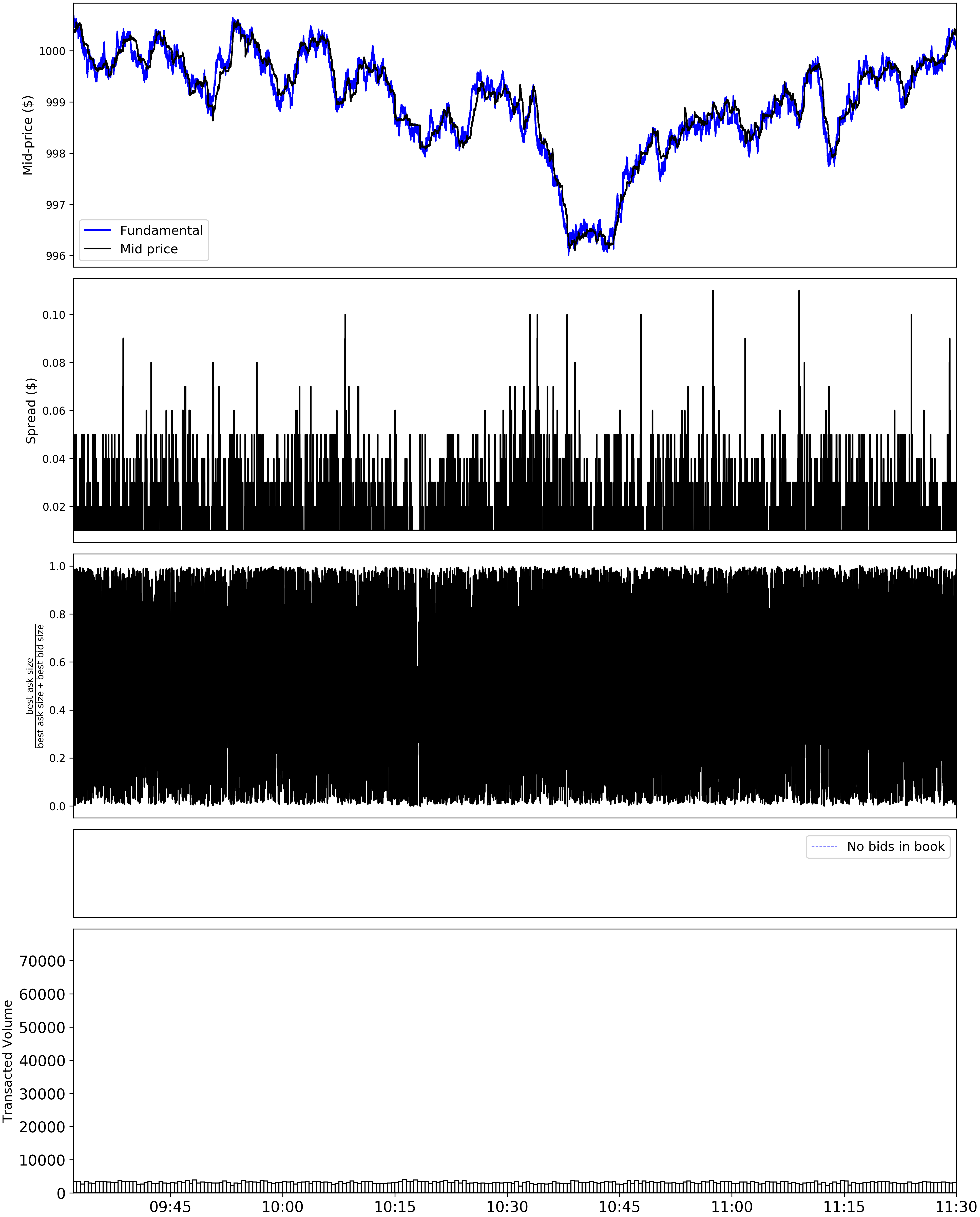
Let's talk through what the above plot shows us.

The top subplot shows the mid-price for the symbol ABM, namely, the half way point between the best bid (offer to buy) and best ask (offer to sell). Also displayed is the value for the fundamental, as seen by the value agents. We see that the mid-price closely tracks the fundamental price. Indeed this is induced by the pressure from the Value Agents. If they see the symbol is mispriced, they will trade in such a way as to take advantage of this, which acts to close the gap between mid-price and fundamental.

The second subplot shows the spread over time for the symbol, defined as the difference between the best bid and best ask. Typically, large tick stocks are those that have a spread of approximately one tick [1], with small tick stocks having a larger spread. For us a large tick stock would mean a spread of one cent. Here ABM has a slightly larger spread; we can think of ABM as being "medium tick".

The third subplot shows participation of volume. This is defined as the number of shares offered at the best ask divided by the sum of shares offered at best bid and best ask. Roughly speaking, a participation of volume close to one means there is more supply for the stock and participation of volume close to zero means there is a lot more demand. Here we see that this quantity is very rapidly oscillating between zero and one as there is a lot of trading happening in the market.

The fourth subplot is empty, and it should be empty! This subplot is there to check that there is sufficient liquidity in the synthetic market, with a vertical line appearing whenever any "liquidity dropout events" occur. These are when one side of the order book is empty, that is, there is no offer at any price to buy (resp. sell) the security.

The bottom subplot shows how much volume is transacted over the day, as in, how many shares are being traded over a unit of time. As ABM is a highly liquid stock we see a large a volume of transactions.

Experimental Agent Config

Now we're placed to run an experimental agent within this config. You'll notice that the configuration has an --execution-agents command-line switch. If activated, this indicates that there will be an additional agent present: an execution agent. One of the benefits of the randomness model in ABIDES is that we can run counterfactual experiments, that is, we can add or remove agents from a simulation run and observe the difference in the synthetic market's behaviour.

The goal of this particular execution agent is to carry out a large order, known as a metaorder. A metaorder is realised by a collection of smaller orders, known as child orders. An example would be a metaorder to buy 10000 shares in ABM, split into 100 child orders, each order comprising a buy order for 100 shares.

The execution order used in the RMSC03 configuration is called a POV execution agent, standing for "percentage of volume". There are other types of execution agent provided in ABIDES, in the agents/execution directory. The POV execution agent is given a target quantity and percentage of volume (POV). At each wakeup, the agent queries the exchange for the total transacted volume since the last wakeup, then places an order with size pov * transacted_volume. The agent stops when the metaorder is fulfilled, although the implementation in ABIDES allows the agent to stop at a specified time also for experimental purposes. Naturally, a larger POV will result in a faster metaorder execution and a smaller POV will be slower. However, a larger POV will have a larger impact on the mid-price as the agent's transactions take up a larger proportion of traded volume.

Single day comparison plot at multiple POV

Using the RMSC03 config we can run a counterfactual experiment: what impact does a POV execution agent have on the synthetic market defined by the RMSC03 config? How does this increase as the POV level increases?

We'll consider the POV agent participating at a number of POV levels: 0.01, 0.05, 0.1 and 0.5. The agent will be executing a buy metaorder over the time period 10:00-11.00.

Note that you'll need the free command-line utility GNU parallel to run the following commands.

for pov in  0.01 0.05 0.1 0.5; do
    sem -j${NUM_JOBS} --line-buffer python -u abides.py -c rmsc03 -t ABM -d 20200603 -s 1234 -l rmsc03_two_hour_pov_${pov} -e -p ${pov}
done

where ${NUM_JOBS} specifies how many jobs to run in parallel. You can change this depending on your computational resources.

Single day plot

We can use another plotting utility to see the effect of the execution agent on this particular day.

cd realism && python -u impact_single_day_pov.py plot_configs/plot_configs/single_day/rmsc03_demo_single_day.json && cd ..

The output, found in realism/visualizations/rmsc03_two_hour_20200603.png, should look something like this.

The top subplot shows the mid-price with no execution agent (baseline) along with the price series for each participation level. The time period during which the execution is active is shown by the greyed panel. Notice that before the agent is active, the price series at all POV participation levels is the same as the baseline, showing us that the changes in mid-price can be attributed solely to the action of the execution agent.

The bottom subplot shows the same data, but scaled to the baseline mid-price (horizontal line at y = 0). We can see that for the seed chosen, the mid-price impact roughly increases with the POV level.

Aggregated execution experiment

The plot in the previous section corresponds to a single simulation run. In a similar way to real markets, our synthetic market shows a lot of variation over different time periods. As such, to draw strong conclusions about market properties, results from multiple simulations must be aggregated. For our execution experiment, we'll do the same below. Here we'll aggregate over 20 runs at each POV level for brevity, although in practise one should use more samples.

for seed in $(seq 100 120); do
  sem -j${NUM_JOBS} --line-buffer python -u abides.py -c rmsc03 -t ABM -d 20200605 -s ${seed} -l rmsc03_demo_no_${seed}_20200605
  for pov in  0.01 0.05 0.1 0.5; do
      sem -j${NUM_JOBS} --line-buffer python -u abides.py -c rmsc03 -t ABM -d 20200605 -s ${seed} -l rmsc03_demo_yes_${seed}_pov_${pov}_20200605 -e -p ${pov}
  done
done

Multiday subplot

We can use another tool to view the aggregated output of these simulations.

cd realism && python -u impact_multiday_pov.py plot_configs/plot_configs/multiday/rmsc03_demo_multiday.json -n ${NUM_JOBS} && cd ..

There should be 4 files named realism/visualizations/rmsc03_demo_pov_${pov}_multiday.png for pov in (0.01 0.05 0.1 0.5) . They should look like this.

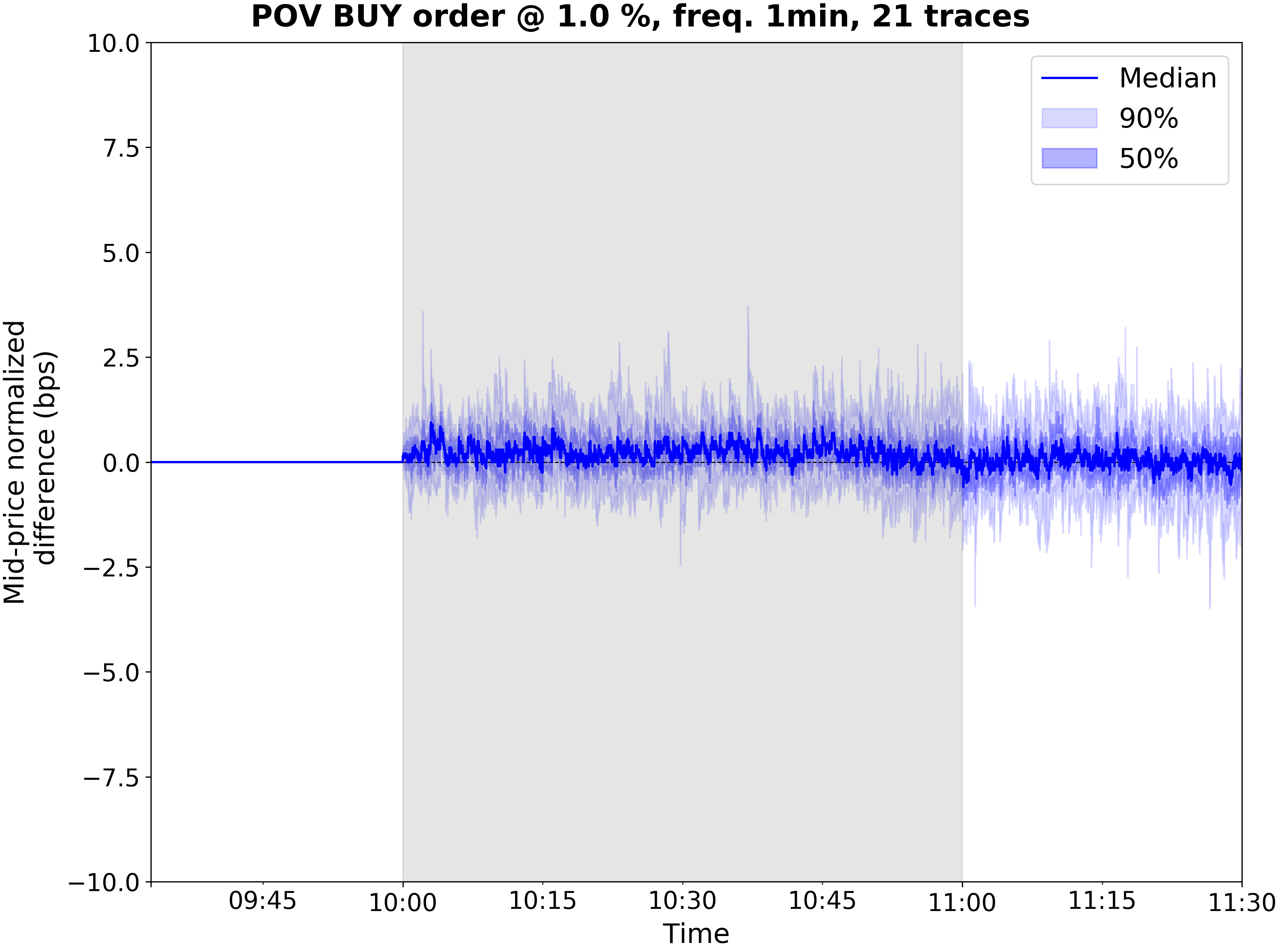
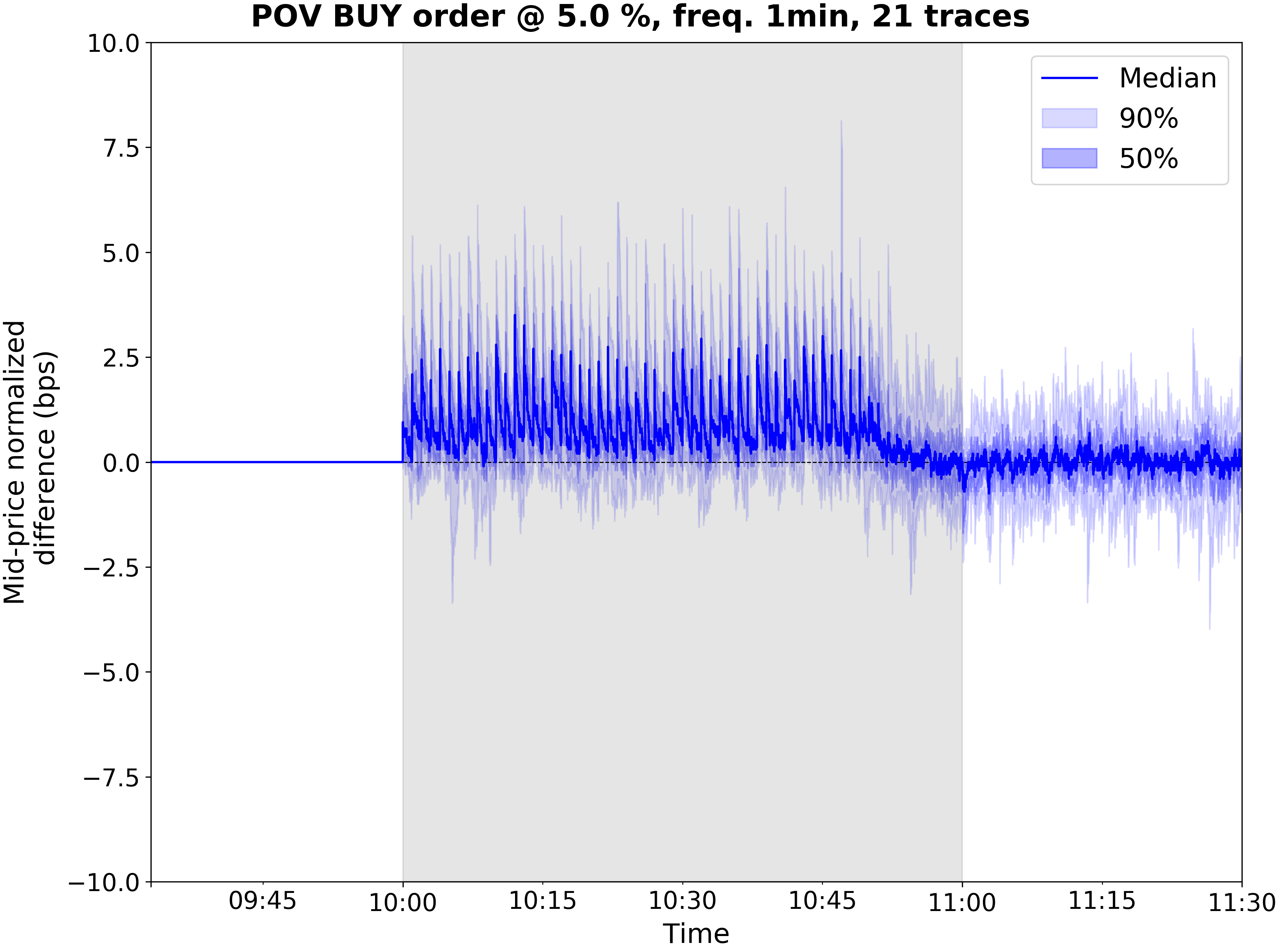
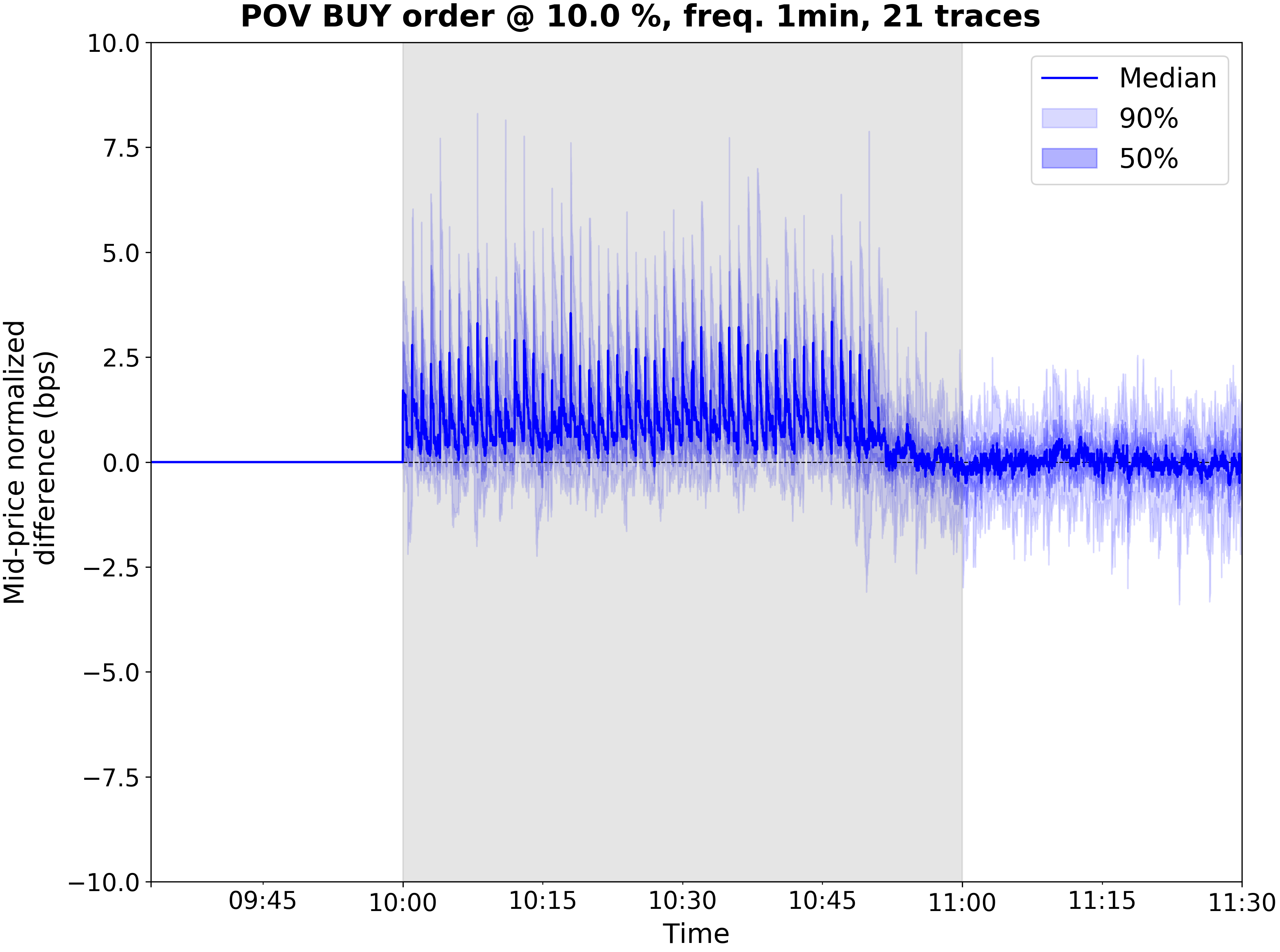
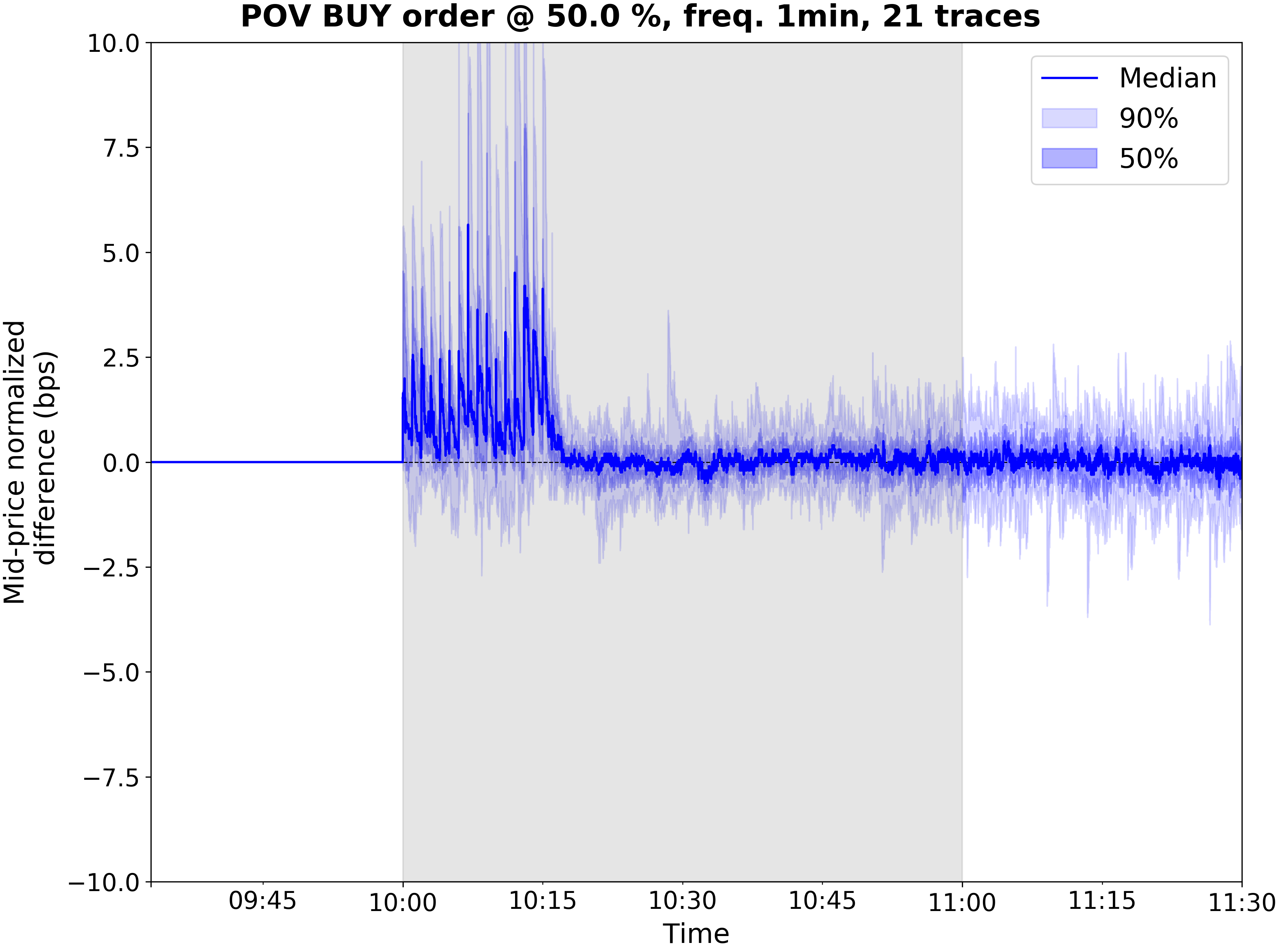
These plots are much like the bottom subplot of the previous subsection -- with the main differences being the POV levels being on separate plots for visibility and uncertainty being quantified by quantile bands around the difference from baseline mid-price. We see that increasing POV increases the average change in mid-price, as one might expect.

Conclusion

In this tutorial we have seen how to run a small counterfactual experiment using the latest reference market simulation configuration (RMSC03) and some of the plotting utilities that allow us to inspect ABIDES simulation results. The best way to learn how to use ABIDES is to take the provided configs and play around with the default parameters. The wiki pages contain lots of further useful information as well. In particular, please see this tutorial on how to build your own trading agent.

Thanks for following along and happy simulating!

====

[Bouchaud_Kockelkoren] The price impact of order book events: market orders, limit orders and cancellations. Zoltan Eisler, Jean-Philippe Bouchaud, Julien Kockelkoren. Quant. Finance, 2012, 12, 1395–1419 arXiv:0904.0900 [q-fin.TR]