---

scikit-posthocs is a Python package that provides post hoc tests for pairwise multiple comparisons that are usually performed in statistical data analysis to assess the differences between group levels if a statistically significant result of ANOVA test has been obtained.

scikit-posthocs is tightly integrated with Pandas DataFrames and NumPy arrays to ensure fast computations and convenient data import and storage.

This package will be useful for statisticians, data analysts, and researchers who use Python in their work.

Background

Python statistical ecosystem comprises multiple packages. However, it still has numerous gaps and is surpassed by R packages and capabilities.

SciPy (version 1.2.0) offers Student, Wilcoxon, and Mann-Whitney tests that are not adapted to multiple pairwise comparisons. Statsmodels (version 0.9.0) features TukeyHSD test that needs some extra actions to be fluently integrated into a data analysis pipeline. Statsmodels also has good helper methods: allpairtest (adapts an external function such as scipy.stats.ttest_ind to multiple pairwise comparisons) and multipletests (adjusts p values to minimize type I and II errors). PMCMRplus is a very good R package that has no rivals in Python as it offers more than 40 various tests (including post hoc tests) for factorial and block design data. PMCMRplus was an inspiration and a reference for scikit-posthocs.

scikit-posthocs attempts to improve Python statistical capabilities by offering a lot of parametric and nonparametric post hoc tests along with outliers detection and basic plotting methods.

Features

• Omnibus tests:
  • Durbin test (for balanced incomplete block design).
  • Mack-Wolfe test.
  • Hayter (OSRT) test.
• Parametric pairwise multiple comparisons tests:
  • Scheffe test.
  • Student T test.
  • Tamhane T2 test.
  • TukeyHSD test.
• Non-parametric tests for factorial design:
  • Conover test.
  • Dunn test.
  • Dwass, Steel, Critchlow, and Fligner test.
  • Mann-Whitney test.
  • Nashimoto and Wright (NPM) test.
  • Nemenyi test.
  • van Waerden test.
  • Wilcoxon test.
• Non-parametric tests for block design:
  • Conover test.
  • Durbin and Conover test.
  • Miller test.
  • Nemenyi test.
  • Quade test.
  • Siegel test.
• Outliers detection tests:
  • Simple test based on interquartile range (IQR).
  • Grubbs test.
  • Tietjen-Moore test.
  • Generalized Extreme Studentized Deviate test (ESD test).
• Other tests:
  • Anderson-Darling test.
• Global null hypothesis tests:
  • Fisher's combination test.
  • Simes test.
• Plotting functionality (e.g. significance plots).

All post hoc tests are capable of p adjustments for multiple pairwise comparisons.

Dependencies

• NumPy and SciPy packages
• Statsmodels
• Pandas
• Matplotlib
• Seaborn

Compatibility

Package is only compatible with Python 3.

Install

You can install the package using pip (from PyPi):

pip install scikit-posthocs

Or using conda (from conda-forge repo):

conda install -c conda-forge scikit-posthocs

The latest version from GitHub can be installed using:

pip install git+https://github.com/maximtrp/scikit-posthocs.git

Examples

Parametric ANOVA with post hoc tests

Here is a simple example of the one-way analysis of variance (ANOVA) with post hoc tests used to compare sepal width means of three groups (three iris species) in iris dataset.

To begin, we will import the dataset using statsmodels get_rdataset() method.

>>> import statsmodels.api as sa
>>> import statsmodels.formula.api as sfa
>>> import scikit_posthocs as sp
>>> df = sa.datasets.get_rdataset('iris').data
>>> df.columns = df.columns.str.replace('.', '')
>>> df.head()
    SepalLength   SepalWidth   PetalLength   PetalWidth Species
0           5.1          3.5           1.4          0.2  setosa
1           4.9          3.0           1.4          0.2  setosa
2           4.7          3.2           1.3          0.2  setosa
3           4.6          3.1           1.5          0.2  setosa
4           5.0          3.6           1.4          0.2  setosa

Now, we will build a model and run ANOVA using statsmodels ols() and anova_lm() methods. Columns Species and SepalWidth contain independent (predictor) and dependent (response) variable values, correspondingly.

>>> lm = sfa.ols('SepalWidth ~ C(Species)', data=df).fit()
>>> anova = sa.stats.anova_lm(lm)
>>> print(anova)
               df     sum_sq   mean_sq         F        PR(>F)
C(Species)    2.0  11.344933  5.672467  49.16004  4.492017e-17
Residual    147.0  16.962000  0.115388       NaN           NaN

The results tell us that there is a significant difference between groups means (p = 4.49e-17), but does not tell us the exact group pairs which are different in means. To obtain pairwise group differences, we will carry out a posteriori (post hoc) analysis using scikits-posthocs package. Student T test applied pairwisely gives us the following p values:

>>> sp.posthoc_ttest(df, val_col='SepalWidth', group_col='Species', p_adjust='holm')
                  setosa    versicolor     virginica
setosa     -1.000000e+00  5.535780e-15  8.492711e-09
versicolor  5.535780e-15 -1.000000e+00  1.819100e-03
virginica   8.492711e-09  1.819100e-03 -1.000000e+00

Remember to use a FWER controlling procedure, such as Holm procedure, when making multiple comparisons. As seen from this table, significant differences in group means are obtained for all group pairs.

Non-parametric ANOVA with post hoc tests

If normality and other assumptions are violated, one can use a non-parametric Kruskal-Wallis H test (one-way non-parametric ANOVA) to test if samples came from the same distribution.

Let's use the same dataset just to demonstrate the procedure. Kruskal-Wallis test is implemented in SciPy package. scipy.stats.kruskal method accepts array-like structures, but not DataFrames.

>>> import scipy.stats as ss
>>> import statsmodels.api as sa
>>> import scikit_posthocs as sp
>>> df = sa.datasets.get_rdataset('iris').data
>>> df.columns = df.columns.str.replace('.', '')
>>> data = [df.loc[ids, 'SepalWidth'].values for ids in df.groupby('Species').groups.values()]

data is a list of 1D arrays containing sepal width values, one array per each species. Now we can run Kruskal-Wallis analysis of variance.

>>> H, p = ss.kruskal(*data)
>>> p
1.5692820940316782e-14

P value tells us we may reject the null hypothesis that the population medians of all of the groups are equal. To learn what groups (species) differ in their medians we need to run post hoc tests. scikit-posthocs provides a lot of non-parametric tests mentioned above. Let's choose Conover's test.

>>> sp.posthoc_conover(df, val_col='SepalWidth', group_col='Species', p_adjust = 'holm')
                  setosa    versicolor     virginica
setosa     -1.000000e+00  2.278515e-18  1.293888e-10
versicolor  2.278515e-18 -1.000000e+00  1.881294e-03
virginica   1.293888e-10  1.881294e-03 -1.000000e+00

Pairwise comparisons show that we may reject the null hypothesis (p < 0.01) for each pair of species and conclude that all groups (species) differ in their sepal widths.

Block design

In block design case, we have a primary factor (e.g. treatment) and a blocking factor (e.g. age or gender). A blocking factor is also called a nuisance factor, and it is usually a source of variability that needs to be accounted for.

An example scenario is testing the effect of four fertilizers on crop yield in four cornfields. We can represent the results with a matrix in which rows correspond to the blocking factor (field) and columns correspond to the primary factor (yield).

The following dataset is artificial and created just for demonstration of the procedure:

>>> data = np.array([[ 8.82, 11.8 , 10.37, 12.08],
                     [ 8.92,  9.58, 10.59, 11.89],
                     [ 8.27, 11.46, 10.24, 11.6 ],
                     [ 8.83, 13.25,  8.33, 11.51]])

First, we need to perform an omnibus test — Friedman rank sum test. It is implemented in scipy.stats subpackage:

>>> import scipy.stats as ss
>>> ss.friedmanchisquare(*data.T)
FriedmanchisquareResult(statistic=8.700000000000003, pvalue=0.03355726870553798)

We can reject the null hypothesis that our treatments have the same distribution, because p value is less than 0.05. A number of post hoc tests are available in scikit-posthocs package for unreplicated block design data. In the following example, Nemenyi's test is used:

>>> import scikit_posthocs as sp
>>> sp.posthoc_nemenyi_friedman(data)
          0         1         2         3
0 -1.000000  0.220908  0.823993  0.031375
1  0.220908 -1.000000  0.670273  0.823993
2  0.823993  0.670273 -1.000000  0.220908
3  0.031375  0.823993  0.220908 -1.000000

This function returns a DataFrame with p values obtained in pairwise comparisons between all treatments. One can also pass a DataFrame and specify the names of columns containing dependent variable values, blocking and primary factor values. The following code creates a DataFrame with the same data:

>>> data = pd.DataFrame.from_dict({'blocks': {0: 0, 1: 1, 2: 2, 3: 3, 4: 0, 5: 1, 6:
2, 7: 3, 8: 0, 9: 1, 10: 2, 11: 3, 12: 0, 13: 1, 14: 2, 15: 3}, 'groups': {0:
0, 1: 0, 2: 0, 3: 0, 4: 1, 5: 1, 6: 1, 7: 1, 8: 2, 9: 2, 10: 2, 11: 2, 12: 3,
13: 3, 14: 3, 15: 3}, 'y': {0: 8.82, 1: 8.92, 2: 8.27, 3: 8.83, 4: 11.8, 5:
9.58, 6: 11.46, 7: 13.25, 8: 10.37, 9: 10.59, 10: 10.24, 11: 8.33, 12: 12.08,
13: 11.89, 14: 11.6, 15: 11.51}})
>>> data
    blocks  groups      y
0        0       0   8.82
1        1       0   8.92
2        2       0   8.27
3        3       0   8.83
4        0       1  11.80
5        1       1   9.58
6        2       1  11.46
7        3       1  13.25
8        0       2  10.37
9        1       2  10.59
10       2       2  10.24
11       3       2   8.33
12       0       3  12.08
13       1       3  11.89
14       2       3  11.60
15       3       3  11.51

This is a melted and ready-to-use DataFrame. Do not forget to pass melted argument:

>>> sp.posthoc_nemenyi_friedman(data, y_col='y', block_col='blocks', group_col='groups', melted=True)
          0         1         2         3
0 -1.000000  0.220908  0.823993  0.031375
1  0.220908 -1.000000  0.670273  0.823993
2  0.823993  0.670273 -1.000000  0.220908
3  0.031375  0.823993  0.220908 -1.000000

Data types

Internally, scikit-posthocs uses NumPy ndarrays and pandas DataFrames to store and process data. Python lists, NumPy ndarrays, and pandas DataFrames are supported as input data types. Below are usage examples of various input data structures.

Lists and arrays

>>> x = [[1,2,1,3,1,4], [12,3,11,9,3,8,1], [10,22,12,9,8,3]]
>>> # or
>>> x = np.array([[1,2,1,3,1,4], [12,3,11,9,3,8,1], [10,22,12,9,8,3]])
>>> sp.posthoc_conover(x, p_adjust='holm')
          1         2         3
1 -1.000000  0.057606  0.007888
2  0.057606 -1.000000  0.215761
3  0.007888  0.215761 -1.000000

You can check how it is processed with a hidden function __convert_to_df():

>>> sp.__convert_to_df(x)
(    vals  groups
 0      1       1
 1      2       1
 2      1       1
 3      3       1
 4      1       1
 5      4       1
 6     12       2
 7      3       2
 8     11       2
 9      9       2
 10     3       2
 11     8       2
 12     1       2
 13    10       3
 14    22       3
 15    12       3
 16     9       3
 17     8       3
 18     3       3, 'vals', 'groups')

It returns a tuple of a DataFrame representation and names of the columns containing dependent (vals) and independent (groups) variable values.

Block design matrix passed as a NumPy ndarray is processed with a hidden __convert_to_block_df() function:

>>> data = np.array([[ 8.82, 11.8 , 10.37, 12.08],
                     [ 8.92,  9.58, 10.59, 11.89],
                     [ 8.27, 11.46, 10.24, 11.6 ],
                     [ 8.83, 13.25,  8.33, 11.51]])
>>> sp.__convert_to_block_df(data)
(    blocks groups      y
 0        0      0   8.82
 1        1      0   8.92
 2        2      0   8.27
 3        3      0   8.83
 4        0      1  11.80
 5        1      1   9.58
 6        2      1  11.46
 7        3      1  13.25
 8        0      2  10.37
 9        1      2  10.59
 10       2      2  10.24
 11       3      2   8.33
 12       0      3  12.08
 13       1      3  11.89
 14       2      3  11.60
 15       3      3  11.51, 'y', 'groups', 'blocks')

DataFrames

If you are using DataFrames, you need to pass column names containing variable values to a post hoc function:

>>> import statsmodels.api as sa
>>> import scikit_posthocs as sp
>>> df = sa.datasets.get_rdataset('iris').data
>>> df.columns = df.columns.str.replace('.', '')
>>> sp.posthoc_conover(df, val_col='SepalWidth', group_col='Species', p_adjust = 'holm')

val_col and group_col arguments specify the names of the columns containing dependent (response) and independent (grouping) variable values.

Significance plots

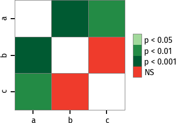
P values can be plotted using a heatmap:

>>> pc = sp.posthoc_conover(x, val_col='values', group_col='groups')
>>> heatmap_args = {'linewidths': 0.25, 'linecolor': '0.5', 'clip_on': False, 'square': True, 'cbar_ax_bbox': [0.80, 0.35, 0.04, 0.3]}
>>> sp.sign_plot(pc, **heatmap_args)

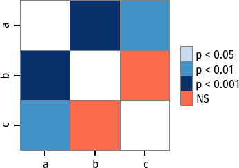
Custom colormap applied to a plot:

>>> pc = sp.posthoc_conover(x, val_col='values', group_col='groups')
>>> # Format: diagonal, non-significant, p<0.001, p<0.01, p<0.05
>>> cmap = ['1', '#fb6a4a',  '#08306b',  '#4292c6', '#c6dbef']
>>> heatmap_args = {'cmap': cmap, 'linewidths': 0.25, 'linecolor': '0.5', 'clip_on': False, 'square': True, 'cbar_ax_bbox': [0.80, 0.35, 0.04, 0.3]}
>>> sp.sign_plot(pc, **heatmap_args)

Citing

If you want to cite scikit-posthocs, please refer to the publication in the Journal of Open Source Software:

Terpilowski, M. (2019). scikit-posthocs: Pairwise multiple comparison tests in Python. Journal of Open Source Software, 4(36), 1169, https://doi.org/10.21105/joss.01169

@ARTICLE{Terpilowski2019,
  title    = {scikit-posthocs: Pairwise multiple comparison tests in Python},
  author   = {Terpilowski, Maksim},
  journal  = {The Journal of Open Source Software},
  volume   = {4},
  number   = {36},
  pages    = {1169},
  year     = {2019},
  doi      = {10.21105/joss.01169}
}

Acknowledgement

Thorsten Pohlert, PMCMR author and maintainer