ControlSystems.jl

A control systems design toolbox for Julia.

Installation

To install, in the Julia REPL:

using Pkg; Pkg.add("ControlSystems")

News

2022-02

• Breaking: Plots.jl is no longer loaded by ControlSystems.jl. This improves loading times for the package, but means that users will have to run using Plots manually before plotting functions are available.
• Deprecations: Functions dare/dlyap/dkalman/dlqr are now deprecated in favor of an interface that uses dispatch on the types Continuous / Discrete. Example: dare(A,B,Q,R) is now are(Discrete,A,B,Q,R) or are(sysd,Q,R).

2021-11

• Time-domain simuations now return a result structure (non breaking)
• Breaking: lsimplot, stepplot, impulseplot have been replaced by plot(lsim()) etc.
• Breaking: pole, tzero has been renamed to their plural form, poles, tzeros.
• Breaking: c2d now no longer returns the x0map for statespace systems, see function c2d_x0map for the old behavior.
• Breaking: The array layout of time and frequency responses has been transposed, i.e., in y,t,x,u = lsim(sys, ...), the output arrays y,x,u are now of shape size(y) == (sys.ny, T).
• New functions observer_controller, observer_predictor, placePI.
• Breaking: The type LQG has been removed, see RobustAndOptimalControl.jl for its replacement.
• Breaking: balreal and baltrunc return an additional value, the applied similarity transform.
• A large set of bug fixes
• For a full list of changes, see here.

Documentation

All functions have docstrings, which can be viewed from the REPL, using for example ?tf .

A documentation website is available at http://juliacontrol.github.io/ControlSystems.jl/latest/.

Some of the available commands are:

Constructing systems

ss, tf, zpk

Analysis

poles, tzeros, norm, hinfnorm, linfnorm, ctrb, obsv, gangoffour, margin, markovparam, damp, dampreport, zpkdata, dcgain, covar, gram, sigma, sisomargin

Synthesis

are, lyap, lqr, place, leadlink, laglink, leadlinkat, rstd, rstc, dab, balreal, baltrunc

PID design

pid, stabregionPID, loopshapingPI, pidplots

Time and Frequency response

step, impulse, lsim, freqresp, evalfr, bode, nyquist

Plotting

lsimplot, stepplot, impulseplot, bodeplot, nyquistplot, sigmaplot, marginplot, gangoffourplot, pidplots, pzmap, nicholsplot, pidplots, rlocus, leadlinkcurve

Other

minreal, sminreal, c2d

Usage

This toolbox works similar to that of other major computer-aided control systems design (CACSD) toolboxes. Systems can be created in either a transfer function or a state space representation. These systems can then be combined into larger architectures, simulated in both time and frequency domain, and analyzed for stability/performance properties.

Example

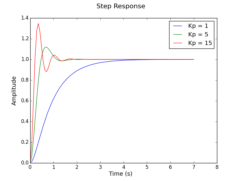
Here we create a simple position controller for an electric motor with an inertial load.

using ControlSystems

# Motor parameters
J = 2.0
b = 0.04
K = 1.0
R = 0.08
L = 1e-4

# Create the model transfer function
s = tf("s")
P = K/(s*((J*s + b)*(L*s + R) + K^2))
# This generates the system
# TransferFunction:
#                1.0
# ---------------------------------
# 0.0002s^3 + 0.160004s^2 + 1.0032s
#
#Continuous-time transfer function model

# Create an array of closed loop systems for different values of Kp
CLs = TransferFunction[kp*P/(1 + kp*P) for kp = [1, 5, 15]];

# Plot the step response of the controllers
# Any keyword arguments supported in Plots.jl can be supplied
using Plots
plot(step.(CLs, 5), label=["Kp = 1" "Kp = 5" "Kp = 15"])

Additional examples

See the examples folder and ControlExamples.jl