Before we get started, we need to install several applications for working with network data. Today, we will be using Sublime Text, Gephi, and R, along with a few of their packages.
Sublime Text is a cross-platform text editor that provides flexible handling of large text files:
We will be using Gephi for network visualization:
Gephi requires that the Java Runtime Environment (JRE). If the JRE is not already installed on your computer, download it here:
If you need to know whether you are running the 32-bit (x86) or 64-bit (x64), use this pointer.
For data analysis, we will be using R:
A nice Integrated Development Environment (IDE) for R can be found here:
For our first network, we will investigate a co-acting network generated using data from the Internet Movie Database (IMDB). In our co-acting network, the nodes will correspond to actors, and an edge will exist between two nodes (actors) if the actors appeared in one or more movies together.

Explore: What sort of questions might we answer using co-acting network? About actors? About genres? About different eras of film?
The data we will use originated here. The entire data set consists of a bipartite network of actors and movies, where actors are connected to movies if the actor appeared in the movie. This is a bipartite network because the network is partitioned into two types of nodes, actors and movies, and edges only exist between (but not within) the two types of nodes.
This network is very large: it consists of 428440 movies and 896308 actors. For a quick introduction to Gephi, we will consider a subset of the total network. First, we filter the set of movies to only those released in 1994 in the genre of science fiction. Then we further collapse the network via a one-mode projection into the co-acting network we will study.
Begin by opening the actor_net.graphml file in the data folder in Sublime Text. If your computer does not recognize the .graphml file extension, you may need to set the file to Open With Sublime Text. If needed, right-click on the file and select Open With, then select Sublime Text.
A snippet from the actor_net.graphml is below:
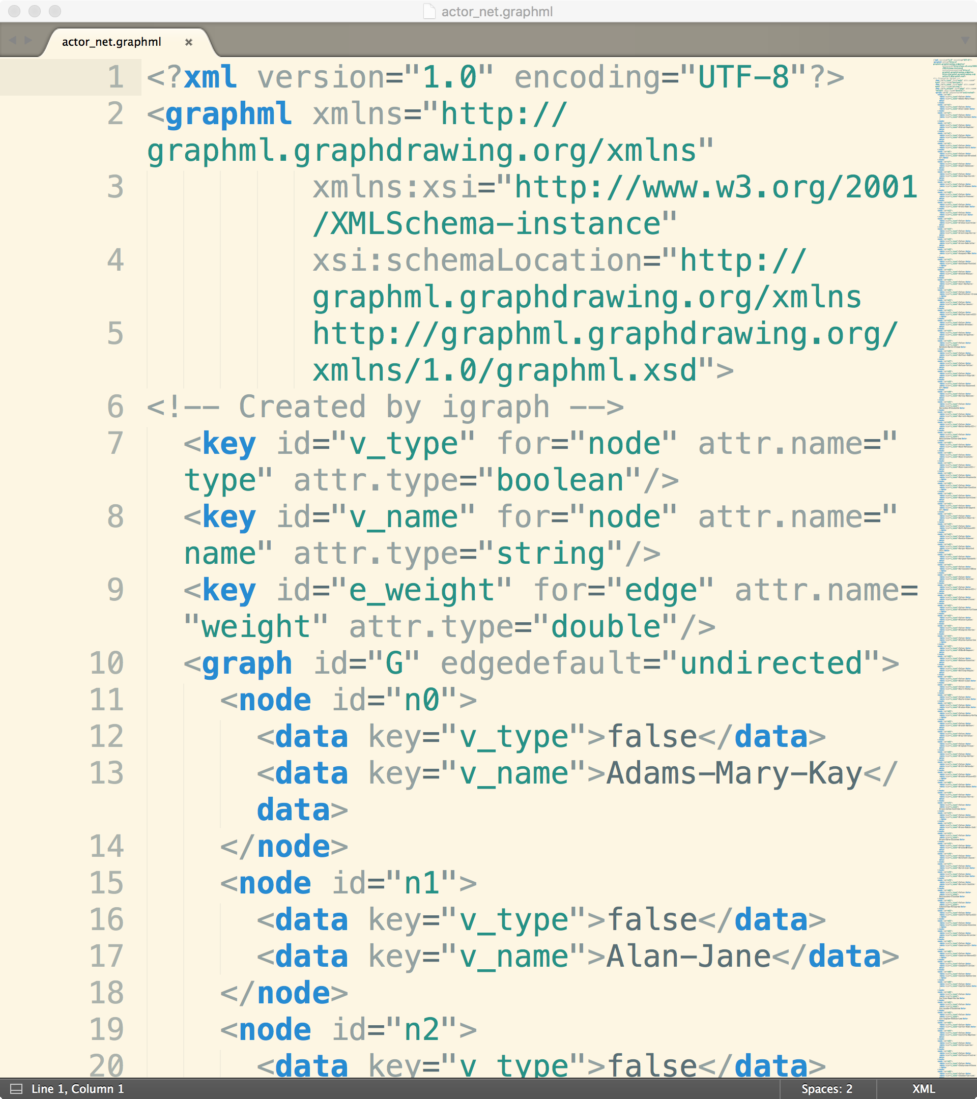
We see that the network is stored in XML format. GraphML is an XML-based network format, with a bit more sophistication than a simple edge list or adjacency matrix. Fortunately, Gephi supports GraphML, among many other formats, so we can load the network into Gephi without knowing the ins-and-outs of the format.
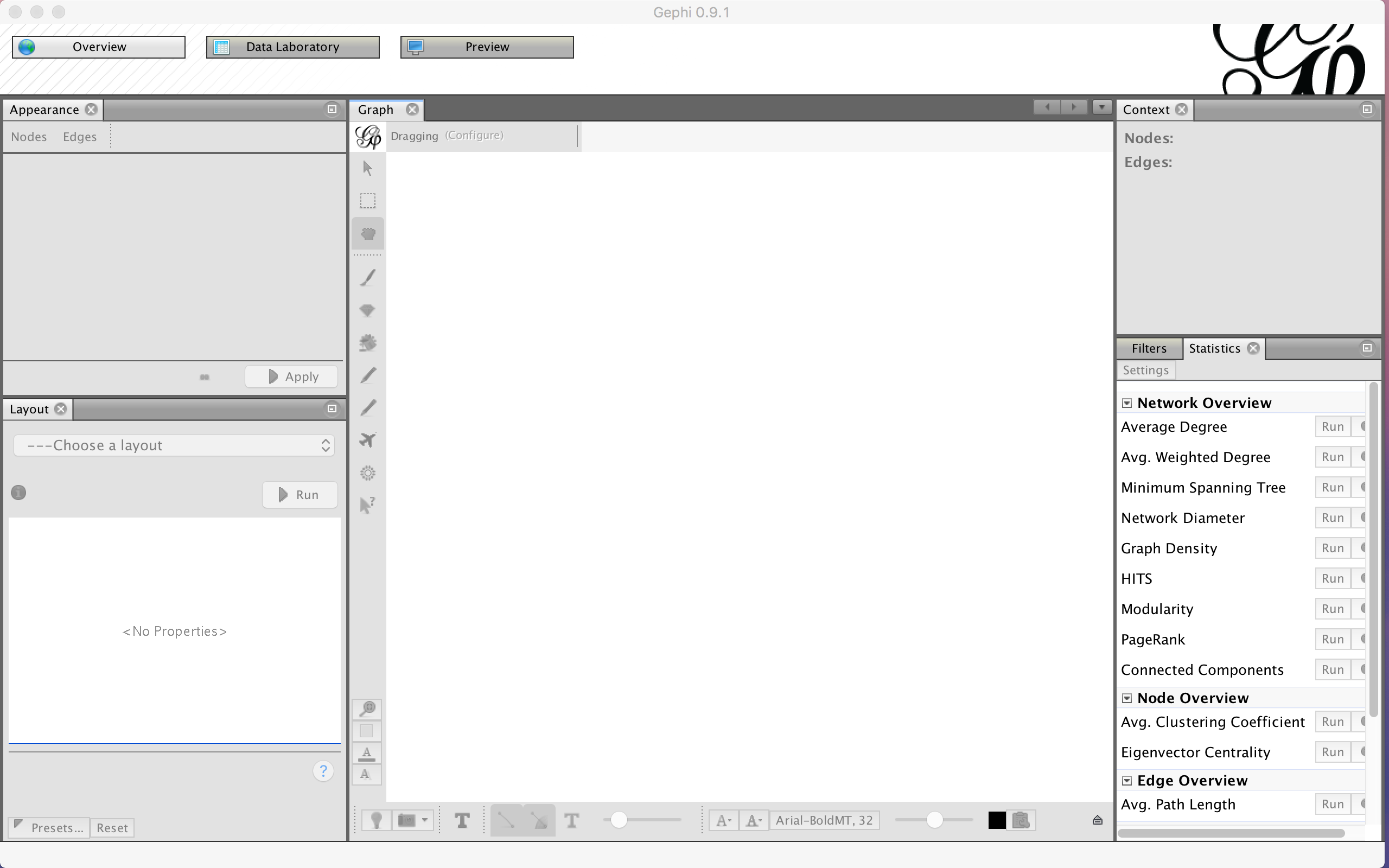
Begin by opening Gephi. After the splash screen closes, you should see a prompt window. Choose New Project. This will lead to a blank Gephi project:
To load the network into Gephi, go to File > Open..., and navigate to folder where you saved the network. This should prompt the import report dialog box:
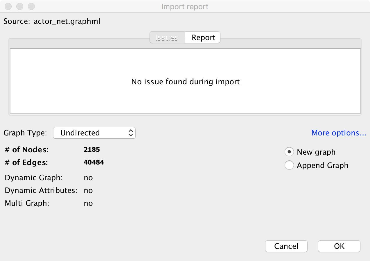
This gives us some details about the network. By default, Gephi is treating the network as undirected, and assumes we have 2185 nodes and 40484 edges. Click OK to load the network into the current Workspace.

We now see the network in the Graph panel of the Overview perspective. If we click over to the Data Laboratory panel, we can see the network from the perspective the Nodes and Edges lists. From this spreadsheet-like perspective, we can filter, sort, etc. on node and edge attributes, as well as add and merge additional columns.
Back in the Graph panel, we see that the network is more-or-less a 'hairball,' a term of art for the naive representation of a network with many nodes and edges. A good first starting point in Gephi is to attempt various different layouts of the network. Gephi has six or so non-trivial network layout algorithms. As a start, run the OpenOrd layout algorithm by choosing OpenOrd from the Layout dropdown menu and clicking Run. Click the magnifying glass in the bottom left corner of the Graph panel to reset the zoom to include the entire network.
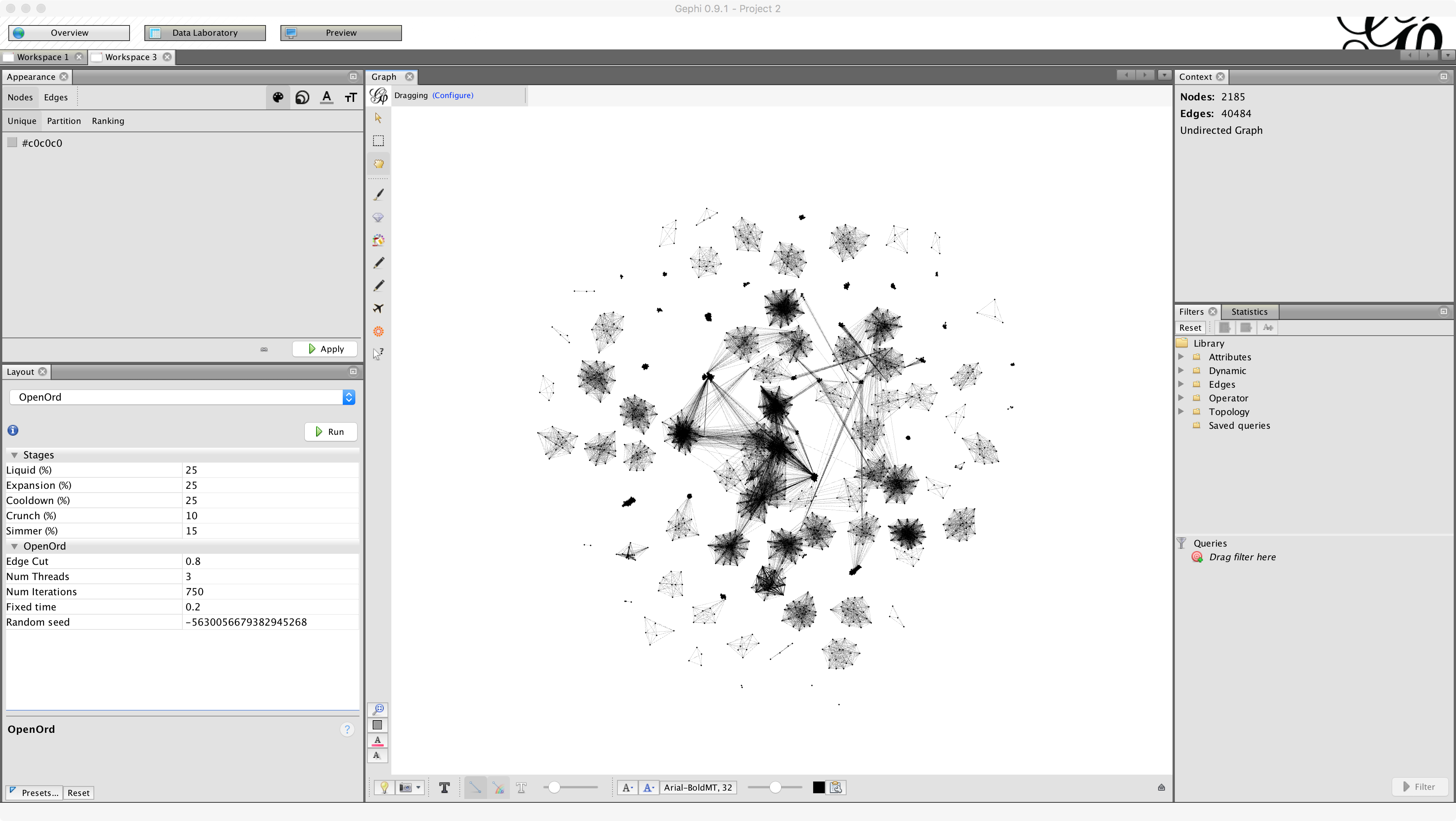
That's better! We can already start to see a good amount of structure in the network. We see several disconnected components in the network.
Explore: Why do we see isolated clusters of actors?
Let's try running another network layout algorithm, this time the Fruchterman-Reingold algorithm. Choose Fruchterman Reingold from the dropdown menu and click Run.
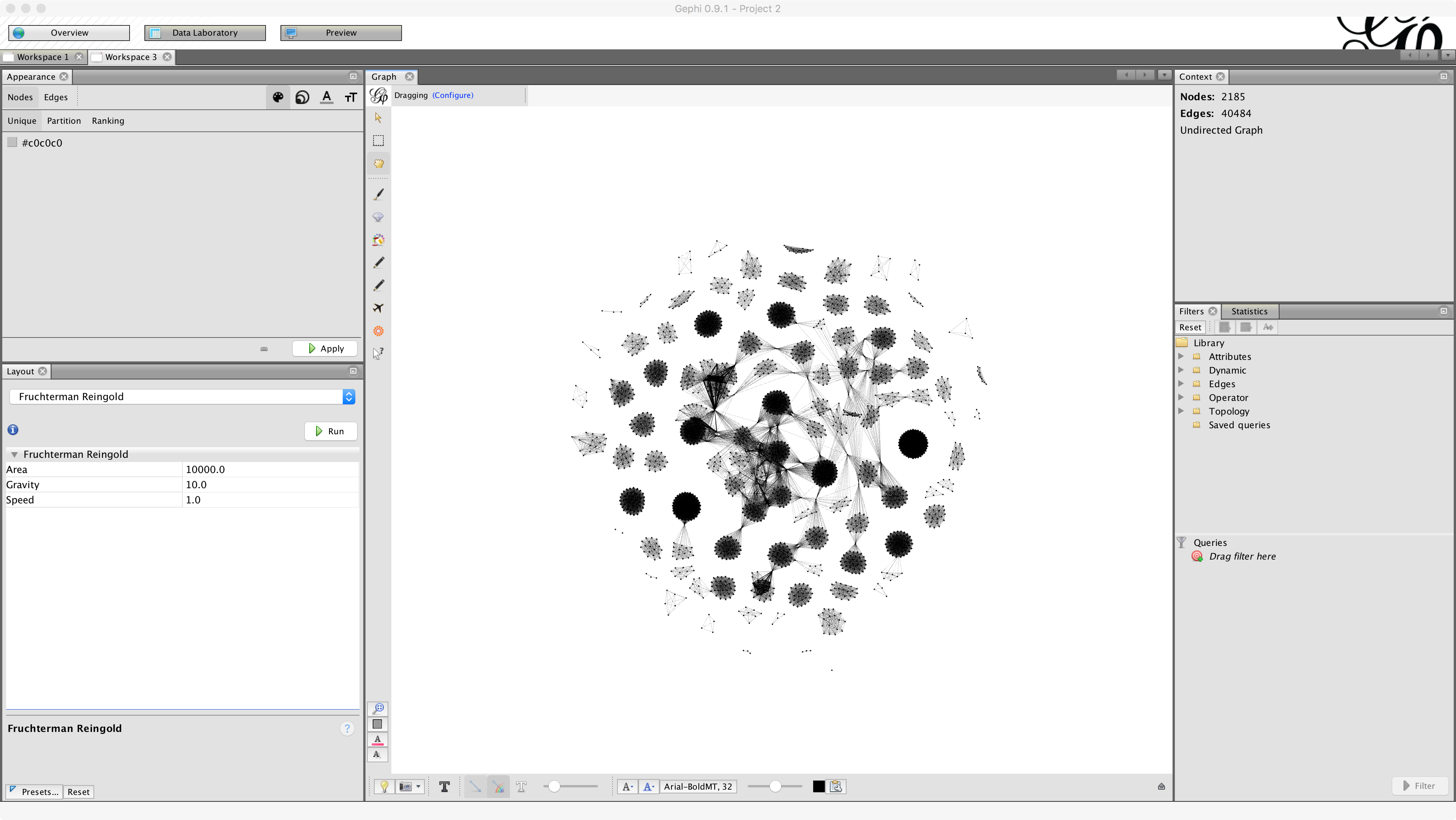
Fruchterman-Reingold is a force-directed layout: that means it treats the the nodes as embedded in a (purely hypothetical!) physical system, where attraction / repulsion between nodes is determined by forces related to the proximity of nodes and whether or not they are connected. See here for more details. We see that after applying Fruchterman-Reingold, some of the clusters have 'relaxed.'
Pointer: If you ever want to 'reset' the layout, you can run Random Layout, which randomly distributes the nodes of the network in a prescribed volume of space. Then you can run the desired layout algorithm 'from scratch.'
Now that we have gotten a feeling for the macro-scale structure of the network, let's compute some of the network statistics we heard about in the talks earlier today. Gephi provides a suite of statistics in the right hand Statistics panel:
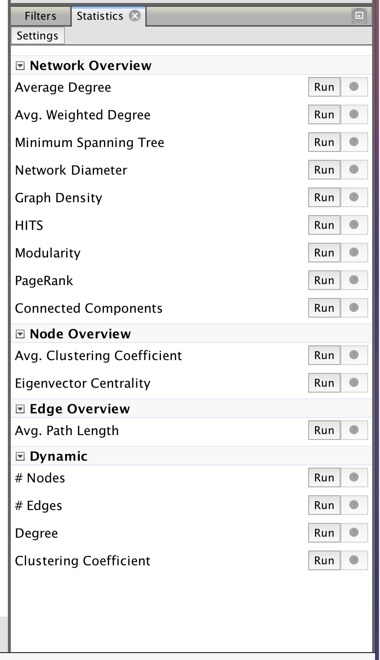
For example, click Run next to Average Degree to compute the degree distribution of the network:
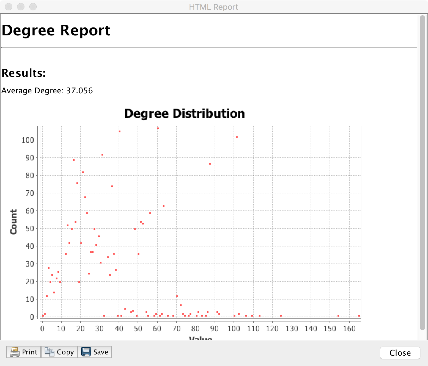
Explore: Does the degree distribution look like a 'power law'? How would you tell?
Gephi computes the in-degree and out-degree for each node in the network. After you compute a node-wise statistic, you can view that statistic for each node as a new column in the Data Laboratory panel:

You can also use node statistics to update the appearance of the network in the Overview panel. To rescale the nodes according to their degree, choose the Node Size icon in the Appearance panel, select the Ranking option, and set the dropdown menu to degree. Change the Max Size option to 40, and click Apply.

To emphasize the nodes over the edges, reduce the width of the edges using the slider in the bottom next to the capital T.

We see that the node sizes (and thus node degrees) are relatively homogeneous within an isolated cluster (why?), but that several 'bridge' nodes have larger degrees relative to their neighbors in the network. Let's select one of these bridge nodes to investigate its identity. To do so, select the Node Investigation pointer in the left pane of the Graph panel, and click on one of the bridge nodes:
Tip: To zoom in and out, use the scroll wheel on your mouse / the two finger swipe on your trackpad. On a Windows computer, use Right Click to drag. On a Mac, use Control-Click to drag.

We see that the bridge node corresponds to William Shatner. He appeared in several sci-fi movies in 1994, amongst them Star Trek: Generations.
Explore: Can you identify which cluster corresponds to the actors from Star Trek: Generations? To find Shatner's neighbors in the network, right click on his entry in the Data Laboratory and choose 'Select neighbour nodes on table'.
Degree is just one of many possible node centralities. A node has large degree centrality if it is connected to many other nodes in the network. Another form of node centrality is eigenvector centrality. A node with high eigenvector centrality has a lot of connections to other nodes that also have many connections.
Explore: Compute the eigenvector centrality of the nodes in the network using the appropriate option in the Statistics panel. How do the eigenvector centralities compare to the degree centralities? Resize the nodes using the eigenvector centralities, and compare the nodes that stand out under each centrality.
Gephi is a great tool for visualizing and analyzing a network. If you are familiar with a scripting langauge (R, Python, Matlab, Octave, Julia, etc.), a great place to get started is with igraph. igraph provides a lot of the same functionality as Gephi, but in a scripting environment that makes automating network analysis a snap.
Let's use igraph to rerun some of the analyses we did in gephi with the IMDB network.
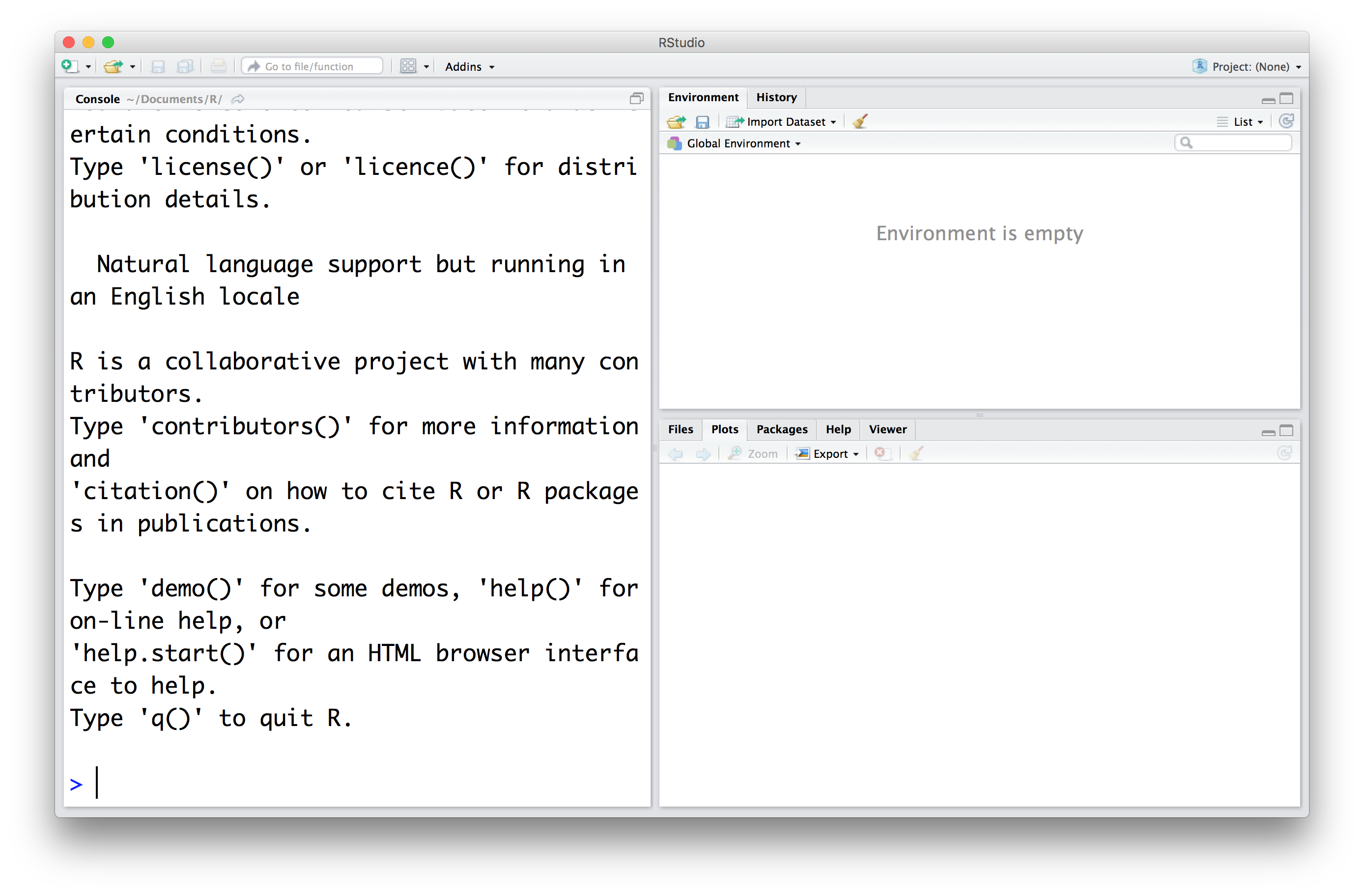
Open RStudio. RStudio is an Integrated Development Environment for R. The IDE includes a Console for active exploration, Environment and History tabs to track variables and previous statements, a File Browser, plotting functionality, debugging and profiling capabilities, and much more.
First, we need to set the working directory to the sfinsc-day1 folder on your machine.
Explore:
In Mac OS, get the path by Option-Right-clicking on sfinsc-day1 and selecting
Copy "sfinsc-day1" as Pathname.In Windows, get the path by Shift-Right-clicking on sfinsc-day1 and selecting
Copy Path. NOTE: Windows uses backslashes (\) between directories, while R expects forward slashes (/). You will have to manually change the backslashes to forward slashes. I suggest using Find & Replace in Sublime Text.
Set the working directory by entering thesetwd function in the Console:
setwd('path/to/sfinsc-day1')
The new working directory is now shown in the top of the Console panel. Click the right arrow at the top of the Console panel to change the file browser to the new directory. Click on the igraph-example.R file to open the script in RStudio. R uses the suffix R for scripts, like c, m, or py for C, Matlab, or Python. The Source Panel now shows the code inside of igraph-example.R.
You can run the code line-by-line in the Console by hitting Control-Enter. The first line of uncommented code installs the igraph package.
install.packages('igraph')
The next lines load the igraph library into R and import the IMDB network, assuming the graphml format.
library(igraph)
network = read_graph("data/imdb/actor_net.graphML", format = 'graphml')
The remaining code uses igraph functions to analyze the network. A list of all igraph functions in R is available here.
NOTE: R, like any programming language, has its quirks:
- R indexes from 1. Not a quirk, per se, but something to keep in mind.
- Periods are treated like any other character, and are often found in function and variable names.
- Assignment to a variable can be done using either the usual '=', or R-specific '->'.
- Members of a list are accessed by the '$' operator. For example, eigen_centrality returns a list with three members: vector, value, and options. To access the (eigen)vector, we use eigen_centrality.out$vector to access the vector member of the list eigen_centrality.out.
With these in mind, let's explore some of the functionality of igraph.
Explore: Running the remaining code in
igraph-example.R, and compare to the statistics computed by Gephi.
To further hone your skills at Network Data Analysis and Gephi, choose between two data sets: correlation networks for S&P 500 companies and co-voting networks from the US Senate.
Start here.
Start here.
The discipline of Network Science is huge, and continually growing. See the Awesome Network Analysis page curated by François Briatte for a list of (almost) all things networks. And then from there, follow links of links of links of... Well, you get the idea.