Python package containing tools for radial basis function (RBF) applications. Applications include interpolating scattered data and solving partial differential equations (PDEs) over irregular domains. Much of this package was inspired by the books "A Primer on Radial Basis Functions with Applications to the Geosciences" by Bengt Fornberg and Natasha Flyer and "Meshfree Approximation Methods with Matlab" by Gregory Fasshauer. The complete documentation for this package can be found here.
- The
RBFclass, which is used to evaluate RBFs and their exact derivatives - The
RBFInterpolantclass, which is used to interpolate scattered and potentially noisy N-dimensional data. One can also evaluate the exact derivatives of the interpolant - The
weight_matrixfunction, which generates radial basis function finite difference (RBF-FD) weights. This is used for solving large scale PDEs over irregular domains - Node generation functions, such as
min_energy_nodesandpoisson_disc_nodes, which are used for solving PDEs with the spectral RBF method or the RBF-FD method - Computational geometry functions (e.g. point in polygon testing) for two and three spatial dimensions
- The
GaussianProcessclass, which is used for Gaussian process regression (GPR). GPR is similar to RBF interpolation, except it has a Bayesian statistical foundation
RBF requires the following packages: numpy, scipy, sympy, cython, and rtree. These dependencies should all be installable with conda or pip.
Download the RBF package
$ git clone http://github.com/treverhines/RBF.gitCompile and install
$ cd RBF
$ python setup.py install
Test that everything works
$ cd test
$ python -m unittest discover'''
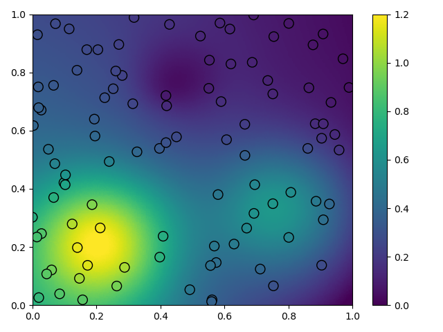
Interpolating scattered observations of Franke's test function with RBFs.
'''
import numpy as np
from rbf.interpolate import RBFInterpolant
import matplotlib.pyplot as plt
np.random.seed(1)
def frankes_test_function(x):
'''A commonly used test function for interpolation'''
x1, x2 = x[:, 0], x[:, 1]
term1 = 0.75 * np.exp(-(9*x1-2)**2/4 - (9*x2-2)**2/4)
term2 = 0.75 * np.exp(-(9*x1+1)**2/49 - (9*x2+1)/10)
term3 = 0.5 * np.exp(-(9*x1-7)**2/4 - (9*x2-3)**2/4)
term4 = -0.2 * np.exp(-(9*x1-4)**2 - (9*x2-7)**2)
y = term1 + term2 + term3 + term4
return y
# observation points
x_obs = np.random.random((100, 2))
# values at the observation points
u_obs = frankes_test_function(x_obs)
# evaluation points
x_itp = np.mgrid[0:1:200j, 0:1:200j].reshape(2, -1).T
interp = RBFInterpolant(x_obs, u_obs)
# interpolated values at the evaluation points
u_itp = interp(x_itp)
# plot the results
plt.tripcolor(
x_itp[:, 0], x_itp[:, 1], u_itp, cmap='viridis', vmin=0.0, vmax=1.2
)
plt.scatter(
x_obs[:, 0], x_obs[:, 1], s=100, c=u_obs, cmap='viridis', vmin=0.0,
vmax=1.2, edgecolor='k'
)
plt.xlim(0, 1)
plt.ylim(0, 1)
plt.colorbar()
plt.tight_layout()
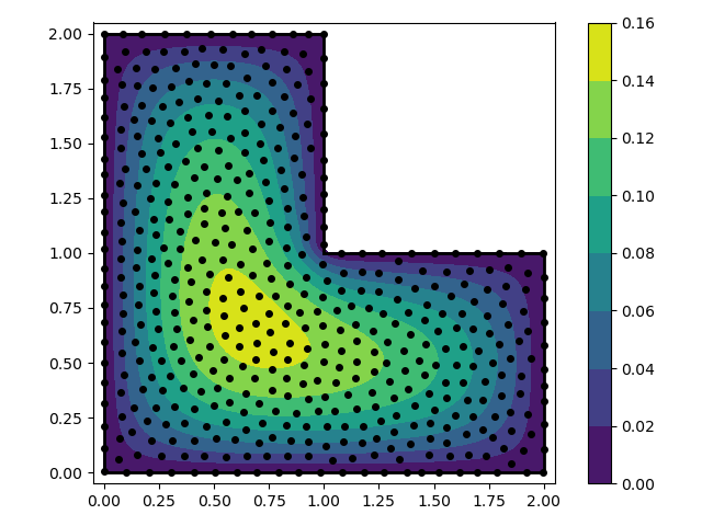
plt.show()There are two methods for solving PDEs with RBFs: the spectral method and the RBF-FD method. The spectral method has been touted as having remarkable accuracy; however it is only applicable for small scale problems and requires a good choice for a shape parameter. The RBF-FD method is appealing because it can be used for large scale problems, there is no need to tune a shape parameter (assuming you use polyharmonic splines to generate the weights), and higher order accuracy can be attained by simply increasing the stencil size or increasing the order of the polynomial used to generate the weights. In short, the RBF-FD method should always be preferred over the spectral RBF method. An example of the two methods is provided below.
'''
In this example we solve the Poisson equation over an L-shaped domain with
fixed boundary conditions. We use the multiquadric RBF (`mq`)
'''
import numpy as np
from rbf.basis import mq
from rbf.pde.geometry import contains
from rbf.pde.nodes import poisson_disc_nodes
import matplotlib.pyplot as plt

# Define the problem domain with line segments.
vert = np.array([[0.0, 0.0], [2.0, 0.0], [2.0, 1.0],
                 [1.0, 1.0], [1.0, 2.0], [0.0, 2.0]])
smp = np.array([[0, 1], [1, 2], [2, 3], [3, 4], [4, 5], [5, 0]])

spacing = 0.07 # approximate spacing between nodes

eps = 0.3/spacing  # shape parameter

# generate the nodes. `nodes` is a (N, 2) float array, `groups` is a dict
# identifying which group each node is in
nodes, groups, _ = poisson_disc_nodes(spacing, (vert, smp))
N = nodes.shape[0]

# create "left hand side" matrix
A = np.empty((N, N))
A[groups['interior']] = mq(nodes[groups['interior']], nodes, eps=eps, diff=[2, 0])
A[groups['interior']] += mq(nodes[groups['interior']], nodes, eps=eps, diff=[0, 2])
A[groups['boundary:all']] = mq(nodes[groups['boundary:all']], nodes, eps=eps)

# create "right hand side" vector
d = np.empty(N)
d[groups['interior']] = -1.0 # forcing term
d[groups['boundary:all']] = 0.0 # boundary condition

# Solve for the RBF coefficients
coeff = np.linalg.solve(A, d)

# interpolate the solution on a grid
xg, yg = np.meshgrid(np.linspace(0.0, 2.02, 100),
                     np.linspace(0.0, 2.02, 100))
points = np.array([xg.flatten(), yg.flatten()]).T
u = mq(points, nodes, eps=eps).dot(coeff)
# mask points outside of the domain
u[~contains(points, vert, smp)] = np.nan
# fold the solution into a grid
ug = u.reshape((100, 100))
# make a contour plot of the solution
fig, ax = plt.subplots()
p = ax.contourf(xg, yg, ug, np.linspace(0.0, 0.16, 9), cmap='viridis')
ax.plot(nodes[:, 0], nodes[:, 1], 'ko', markersize=4)
for s in smp:
  ax.plot(vert[s, 0], vert[s, 1], 'k-', lw=2)

ax.set_aspect('equal')
ax.set_xlim(-0.05, 2.05)
ax.set_ylim(-0.05, 2.05)
fig.colorbar(p, ax=ax)
fig.tight_layout()
plt.show()
'''
In this example we solve the Poisson equation over an L-shaped domain with
fixed boundary conditions. We use the RBF-FD method. The RBF-FD method is
preferable over the spectral RBF method because it is scalable and does not
require the user to specify a shape parameter (assuming that we use odd order
polyharmonic splines to generate the weights).
'''
import numpy as np
from scipy.sparse import coo_matrix
from scipy.sparse.linalg import spsolve
import matplotlib.pyplot as plt
from rbf.sputils import expand_rows
from rbf.pde.fd import weight_matrix
from rbf.pde.geometry import contains
from rbf.pde.nodes import poisson_disc_nodes
# Define the problem domain with line segments.
vert = np.array([[0.0, 0.0], [2.0, 0.0], [2.0, 1.0],
[1.0, 1.0], [1.0, 2.0], [0.0, 2.0]])
smp = np.array([[0, 1], [1, 2], [2, 3], [3, 4], [4, 5], [5, 0]])
spacing = 0.07 # approximate spacing between nodes
n = 25 # stencil size. Increase this will generally improve accuracy
phi = 'phs3' # radial basis function used to compute the weights. Odd
# order polyharmonic splines (e.g., phs3) have always performed
# well for me and they do not require the user to tune a shape
# parameter. Use higher order polyharmonic splines for higher
# order PDEs.
order = 2 # Order of the added polynomials. This should be at least as
# large as the order of the PDE being solved (2 in this case). Larger
# values may improve accuracy
# generate nodes
nodes, groups, _ = poisson_disc_nodes(spacing, (vert, smp))
N = nodes.shape[0]
# create the components for the "left hand side" matrix.
A_interior = weight_matrix(
x=nodes[groups['interior']],
p=nodes,
n=n,
diffs=[[2, 0], [0, 2]],
phi=phi,
order=order)
A_boundary = weight_matrix(
x=nodes[groups['boundary:all']],
p=nodes,
n=1,
diffs=[0, 0])
# Expand and add the components together
A = expand_rows(A_interior, groups['interior'], N)
A += expand_rows(A_boundary, groups['boundary:all'], N)
# create "right hand side" vector
d = np.zeros((N,))
d[groups['interior']] = -1.0
d[groups['boundary:all']] = 0.0
# find the solution at the nodes
u_soln = spsolve(A, d)
# Create a grid for interpolating the solution
xg, yg = np.meshgrid(np.linspace(0.0, 2.02, 100), np.linspace(0.0, 2.02, 100))
points = np.array([xg.flatten(), yg.flatten()]).T
# We can use any method of scattered interpolation (e.g.,
# scipy.interpolate.LinearNDInterpolator). Here we repurpose the RBF-FD method
# to do the interpolation with a high order of accuracy
I = weight_matrix(
x=points,
p=nodes,
n=n,
diffs=[0, 0],
phi=phi,
order=order)
u_itp = I.dot(u_soln)
# mask points outside of the domain
u_itp[~contains(points, vert, smp)] = np.nan
ug = u_itp.reshape((100, 100)) # fold back into a grid
# make a contour plot of the solution
fig, ax = plt.subplots()
p = ax.contourf(xg, yg, ug, np.linspace(-1e-6, 0.16, 9), cmap='viridis')
ax.plot(nodes[:, 0], nodes[:, 1], 'ko', markersize=4)
for s in smp:
ax.plot(vert[s, 0], vert[s, 1], 'k-', lw=2)
ax.set_aspect('equal')
ax.set_xlim(-0.05, 2.05)
ax.set_ylim(-0.05, 2.05)
fig.colorbar(p, ax=ax)
fig.tight_layout()
plt.show()

