Final project for the 2020-2021 Postgraduate course on Artificial Intelligence with Deep Learning, UPC School, authored by Enrique González Terceño, Sofia Limon, Gerard Pons and Celia Santos.
Advised by Amanda Duarte.
- INTRODUCTION AND MOTIVATION
- DATASET
- ARCHITECTURE AND RESULTS
- ABLATION STUDIES
- END TO END SYSTEM
- HOW TO
How many times have you been watching TV and couldn't find the remote? Or you are cooking, eating... and your hands are too messy to interact with a device? Or maybe you would simply like to use devices more intuitively. We use gestures every day of our life, as our primary way of interacting with other humans. Our project emerges as a way to interact with devices in an easier, more convenient manner.
We have created a gesture recognition system that works by capturing videos with a camera, to perform basic tasks on a personal device. But our idea is that it can be further developed to different environments, like for virtual assistants or home appliances, or in a car (instead of taking your eyes off the road, you can control the navigation system a gesture and avoid any potential risks), or in a medical environment (for instance for a doctor to explore a radiography in a middle of a surgery).
The data we used to train and validate our model was from the Jester Dataset, which is a label collection of videos of humans performing hand gestures. The data is given in the JPG frames of the videos, which were recorded at 12 fps. Specifically, the dataset contains 150k videos of 27 different classes.
As the goal of our project was to control basic functionalities of a computer, we decided to reduce the number of classes and to choose 9 gestures which made more sense from a control point of view. The used classes and the number of samples of each one are:
| Gesture | Train Samples | Validation Samples |
|---|---|---|
| Doing Other Things | 9592 | 1468 |
| No Gesture | 4287 | 533 |
| Sliding Two Fingers Down | 4348 | 531 |
| Sliding Two Fingers Up | 4219 | 522 |
| Stop Sign | 4337 | 536 |
| Swiping Left | 4162 | 494 |
| Swiping Right | 4084 | 486 |
| Thumb Up | 4373 | 539 |
| Turning Hand Clockwise | 3126 | 385 |
The first two classes, Doing Other Things and No Gesture, were added to our list of classes in order to have basic states when we are not trying to control the computer.
The Jester test set provided is unlabeled, as the purpose of the dataset is to be a Challenge. Hence, as the end goal of the classifier is to be used with user inputs from a webcam, we decided to perform the test phase with videos created by us on the end to end system.
To better understand the model’s architecture, the general pipeline should be first briefly explained. First of all, when an RGB video is received its optical flow is computed and features are extracted from both videos using an I3D Network. Then, these features are fed into a Neural Network, whose output are the probabilities for each class.
It must be noted that the decision of using RGB and Optical Flow videos was made after different attempts to improve the model.
We computed the dense Optical Flow with the Farneback’s algorithm implementation of OpenCV. As the videos of the dataset have a low resolution and experience a lot of lightning changes, the Optical Flow results showed some imperfections, which we tried to solve by different approaches. Unfortunately, we could not find how to correct them, and decided to move on with the Optical Flow we had in order to be able to continue advancing with the project.
In order to extract features from the videos (both RGB and Optical Flow) we used an Inflated 3D Network (I3D), as it is a widely used network for video classification, able to learn spatiotemporal information from the videos. In our case, we have chosen the i3d_resnet50_v1_kinetics400 provided by GluonCV, since it’s an state-of-the-art model with a good balance between accuracy and computational requirements.
The ResNet50 architecture is shown below:
This I3D had weight initialization from a ResNet50 network trained on Imagenet, and afterwards pre-trained on the action recognition dataset Kinetics-400. The model runs on MXnet DL framework.
Each video (RGB and Optical Flow) is fed through this feature extractor obtaining a (1, 2048) tensor as output, which is saved as a numpy file by the feature extractor.
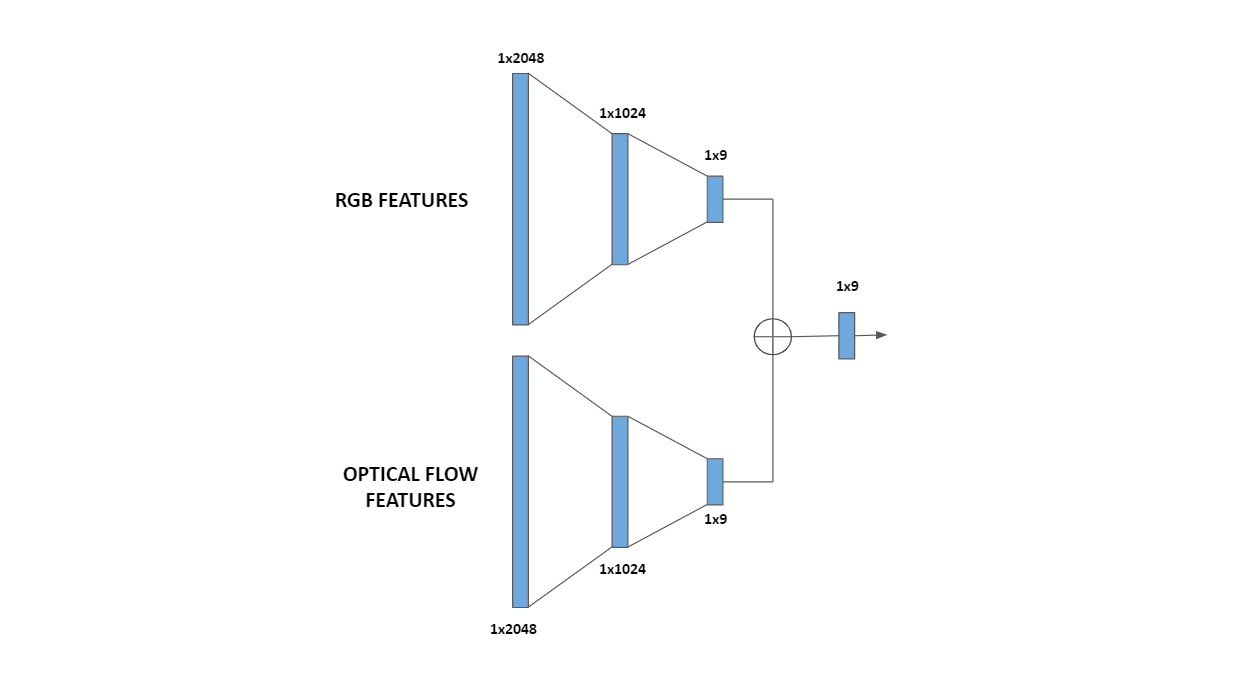
The RGB and the Optical Flow videos are processed by the previously mentioned I3D network, and features for both of them are obtained and go through a neural network architecture with two streams, which was designed considering the different options of how to combine the features. Briefly, both features go through their respective branches of the neural network and the output logits are added up and go through a LogSoftMax layer whose output are the final probabilities. Each branch is made of two fully connected layers with a ReLu activation in between, plus a dropout layer. As loss function we selected Cross-Entropy Loss (that incorporates the final LogSoftMax layer).
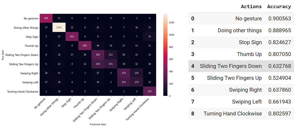
This network was trained and hyperparameter-tuned to yield the final results, whose confusion matrix and accuracy per class are shown below:
This model was saved and used on the final gesture recognition task.
Optical flow is the apparent motion of objects within a video. In our first approach to the model, we saw that where it failed the most was with the movement gestures (non static), and that is why we decided to include explore the optical flow as an input to our model.
Our initial approach was using the Farneback Optical Flow, but as we stated previously, we were not completely satisfied with the result, as there appeared to be a lot of unwanted background "noise". See the following, for example:
The videos in our dataset are of:
- Average quality
- Are a bit grainy
- Can have sudden lighting changes
- Can have a non-homogeneous/moving background
For this reason we decided to try and improve the optical flow detection by trying out different techniques.
Motivation: If we reduce the granularity and the amount of colors in the image, there will be more homogeneity, and less variation within the background lighting. Here we applied gaussian filtering to reduce the noise - or to "smooth" the image - and then an image quantization with 3 values following k-means clustering. Actual result: There is less difference within a single image, but still a big difference between consecutive frames, meaning that it did not improve the optical flow output. In fact, the output was worse than expected:
(Original optical flow on the left, modified optical flow on the right)
Motivation: A big factor in the background noise of the optical flow are the lighting changes. By reducing the luminosity of the image, when calculating the optical flow the background differences won't be so noticeable and the foreground movement will be more prominent. Actual result: On some videos this seemed to work quite well. The moving background, which was our initial main problem, became almost static, and the hand gesture is the only real movement in the image.
(Original optical flow on the left, reduced luminosity optical flow on the right)
However, because of the differences between videos (lighting conditions, uniformity...), the same bitwise operation did not work well for all the videos... sometimes the gesture was not even detected by the optical flow:
Motivation: All we really need from the optical flow is a good representation of the direction of the hand movement. So although sparse optical flow is a vector representation, maybe it could work for our task and better than dense optical flow.
Actual result: It worked very well for a number of videos. See this for example:
But... the algorithm could not be generalized to be applied to all videos. The way sparse optical flow works is that it detects corners within an image, and from that it estimates the movement agains a previous frame.
Using the same parameters as with the previous video, other videos like these ones detected nothing or close to nothing:
Some videos refused to work at all with this method, due to the fact of no points being estimated. Changing the parameters increased the amount of videos that were processed, but reduced the quality of the movement tracking. ''Because of the real-time nature of this project, we cannot rely on trial and error'' If we increased the minimum distance between points, then we wouldn't get an error, but the result for the videos that already worked were not good.
Motivation: Paper "Making Optical Flow Robust to Dynamic Lighting Conditions for Real-Time Operation". The main idea in this paper above is to 1) extract the second derivative, or the laplacian of the image - which finds the edges of an image - then 2) to extract the optical flow from the original image, and finally 3) to isolate the true flow using the laplacian mask created before. Following this approach, our last resource was to apply a mask to the optical flow. An explored methd to find a good mask was applying a gaussian filter to smooth the edges, applying the laplacian filter to detect the contours and using image morphology as a post processing method to clean up the mask. Actual result: The expected results were not the desired ones, as we were unable to create a mask without "holes" or missing sections in the regions of interest.
In conclusion, we did not apply any of these techniques. The objective was trying to remove background noise and keep the main focus on the hand gesture, but none of the tested methods improved the optical flow results.
One of the decisions we had to make is how to join the RGB and Optical Flow, and we explored various possibilities based on the ones mentioned in a paper of action recognition for low resolution videos:
- Addition of the I3D features
- Concatenation of the I3D features
- Maximal value retention for each I3D features
- Addition of the logits from two different networks
The first three methods are based on the use of a single NN to classify the features, whereas the last one uses two different NNs, one for the RGB features and another one for the Optical Flow ones. The method with which the features are joined can have great impact on our network, as the number of layers, network parameters and hyperparameters to tune changes between them, so deciding which one to use was crucial to be able to start with an appropriate training of the network.
Hence, we tested the different methods with similar standard networks. We obtained the results shown on the figure below, and as we can see the performance is quite similar for all of the methods, with the concatenation (Concat) and logit addition (Sum after) methods performing slightly better than the other ones.
To decide which method to use we explored the number of parameters, to try to minimize computational time/cost, and of hyperparameters, to account for the tunability of the model. Regarding the parameters of the networks, both have a very similar number of them, with a difference on parameters of three orders of magnitude lower than the total number of parameters, so it was considered negligible. With respect to the tunability, the method that adds up the logits has nearly the double of hyperparameters as the concatenation method, so we decided to use the former in our architecture.
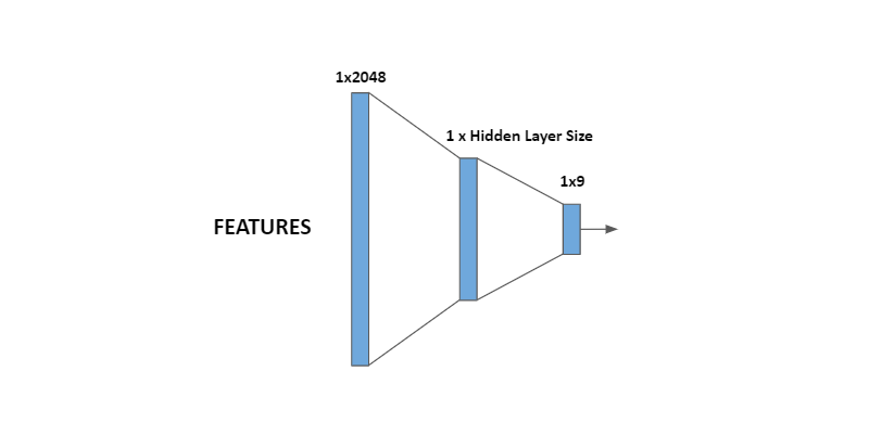
The first way we explored to address the classification task was using only the extracted features from the RGB videos to classify them. We designed a classifier neural network made of two fully connected layers with a ReLu activation in between. As loss function we selected Cross-Entropy Loss since we're solving a classification task:
The first training tests showed that the model overfitted quickly after a few epochs, therefore we added a dropout layer as it enabled the model to learn further.
Next, we performed some basic trainings, changing the value of hyperparameters to see how the model performed. As we had already chosen the activation function (ReLu) and the Loss function (Cross-Entropy Loss), the remainder hyperparameters to be defined were:
- Learning rate
- Batch size
- Number of hidden layers
- Dropout
- Number of epochs
- Optimizer
With respect to the optimizer, we ran trainings with SGD and Adam to compare the results obtained. An example is given below:
 · Optimizers: ADAM, SGD (momentum=0.9, nesterov=True)
 · Learning rate = 1e-3
 · Batch size = 64
 · Number of hidden layers = 1024
 · Dropout = 0.5
 · Number of epochs = 22
As it's clearly seen in the graphs, for the same number of epochs Adam obtained better values in loss and accuracy compared to SGD, although with SGD the curves were smooth and were presumed to get better in the long run. Besides, using Adam made the model overfit before than using SGD, so special care must be taken in choosing dropout value.
At this point we did some hyperparameter tuning to select the best values for our network.
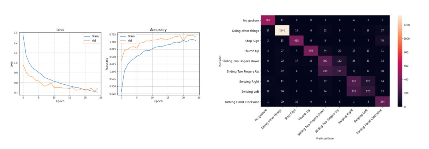
After some training and hyperparameter tuning, the obtained accuracy was around 70%, which was still far from our desired accuracy values. To try to understand better where the model was struggling, we computed the confusion matrix of the predictions and some revealing results where found: the model encountered difficulties when differentiating the gestures that are the same movement but in different directions (i.e. Swiping left/Swiping right) and also differentiating similar gestures which differ from one another mainly by the movement (Stop Sign/Turning Hand Clockwise):
 · Learning rate = 1e-3			· Dropout = 0.5
 · Batch size = 32			· Number of epochs = 25
 · Number of hidden layers = 512	· Optimizer: Adam
To address that problem, we thought that we could capture better the temporal and directional information by computing the Optical Flow of the videos and extract features from them.
After training the model with only the Optical Flow features (following the same steps that had been done during the first approach), it was observed that the accuracy of the whole model diminished, as the model could not classify well the videos with little movement (Stop Sign, Thumb Up). However, the confusion between the troublesome gestures was reduced, confirming the hypothesis that better directional information was captured:
 · Learning rate = 3e-4			· Dropout = 0.5
 · Batch size = 128			· Number of epochs = 25
 · Number of hidden layers = 2048	· Optimizer: Adam
Note : For this training it was used the same Colab notebook than for the first approach, the only change that must be done is loading Flow features pickle file instead of RGB one.
A detailed accuracy comparison between the two approaches can be seen on the table below:
| Gesture | RGB accuracy | FLOW accuracy |
|---|---|---|
| Doing Other Things | 0.954 | 0.795 |
| No Gesture | 0.913 | 0.719 |
| Sliding Two Fingers Down | 0.568 | 0.598 |
| Sliding Two Fingers Up | 0.367 | 0.523 |
| Stop Sign | 0.774 | 0.348 |
| Swiping Left | 0.567 | 0.578 |
| Swiping Right | 0.344 | 0.609 |
| Thumb Up | 0.742 | 0.380 |
| Turning Hand Clockwise | 0.867 | 0.566 |
From the first and second approaches, we decided to use a model with two streams, following the ideas of the Quo Vadis, Action Recognition? paper: we used one stream for RGB videos (spatial stream) to help with the general classification task and the other one for the Optical Flow (temporal stream) to address the confusion problem, and combine them as stated on the previous section. Doing so doubles the amount of data and computer time/cost but was done in the hope of the model being able to keep the best parts of both approaches and yield better results.
In the following trainings we used the best hyperparameters obtained as explained in the hyperparameter section, and applied them symmetrically to both streams (using this Colab notebook):
| Parameter | Value Range |
|---|---|
| Learning Rate | 0.000178044 |
| Batch Size | 64 |
| RGB Hidden Layer | 1024 |
| Flow Hidden Layer | 1024 |
In the first two-stream training tests we continued using Adam optimizer and got these results with dropout = 0.5 and 20 epochs:
As it can be observed on the figure, our hypothesis was true and the network managed to learn appropriately from the two streams of data and improved the overall accuracy, which went from 70% of the RGB videos and 57% of the Optical Flow ones up to +80%, a significant increase.
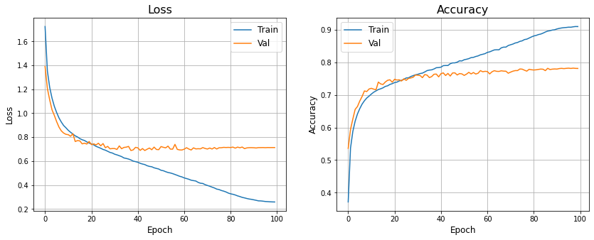
Then, we tried to explore by increasing dropout value making thus possible to increase the number of epochs likewise. An execution example can be seen below, with dropout = 0.75 and 100 epochs:
Taking a look at validation loss' values it can be seen that overfitting occurs for epoch > 70.
At this point we wanted to explore if we could improve a bit more the training by using an scheduler, and we chose OneCycleLR, since it uses a interesting learning rate policy (going from an initial learning rate to some maximum learning rate and then from that maximum learning rate to some minimum learning rate much lower than the initial learning rate).
Our first attempt wasn't successful, as the combination of Adam + OneCycleLR showed to be unsuccessful, at least with the hyperparameters used. Overfitting is observed from right the beginning (with dropout = 0.7):
Then we switched back to SGD optimizer expecting that it was more compatible with OneCycleLR scheduler, supposition that turned to be right. These are the loss and accuracy graphs obtained with a dropout value of 0.5 (using this Colab notebook):
Zooming the graph to detect overfitting showed than overfitting began approximately after epoch 86, so we saved model_state_dict at epoch 81 to be used to infer gestures from video in the app implementation:
In summary, the best model we found achieved a 83.11% accuracy and was obtained using SGD optimizer, OneCycleLR scheduler and the following hyperparameters:
| Hyperparameter | Value |
|---|---|
| Learning Rate | 0.000178044 |
| Batch Size | 64 |
| RGB Hidden Layer | 1024 |
| Flow Hidden Layer | 1024 |
| Dropout | 0.5 |
However, it must be noted that, although there is an increase in the overall accuracy with the two-stream model, the final individual accuracies are an intermediate value between those of the first and the second approaches, in such a way that 'static' classes (as 'thumb up') get worse compared to the RGB model, while 'dynamic' ones (as sliding or swiping) get better.
To try to get the best results possible, an extensive hyperparameter tuning was performed.
To do this we used Ray Tune, a convenient Python library for experiment execution and hyperparameter tuning at any scale.
As choosing dropout value depends on the optimizer used and number of epochs, we used Tune to determine only the following hyperparameters:
- Learning rate
- Batch size
- Number of hidden layers
The range of values tuned for each hyperparameter was as follows:
| Parameter | Value Range |
|---|---|
| Learning Rate | (1e-4 , 1e-2) |
| Batch Size | 8, 16, 32, 64, 128, 256 |
| Hidden Layer size | 128, 256, 512, 1024, 2048 |
As scheduler we chose ASHA (Asynchronous HyperBand Scheduler), since this implementation provides better parallelism and avoids straggler issues during eliminations compared to the original version of HyperBand. We wanted to leverage its ability to perform early stopping (stop automatically bad trials), although at the end we didn't manage to make it work.
First of all, we ran it only with RGB videos (first approach) with 50 samples (number of trials), with Adam optimizer and a dropout = 0.5 and 20 epochs as fixed values. Check Colab notebook here. The best values (*) found were:
- 'lr': 0.00023202085501207852
- 'batch_size': 64,
- 'hidden_size': 1024
obtaining
- Best trial final validation loss: 0.6756827401560407
- Best trial final validation accuracy: 0.7360640168190002
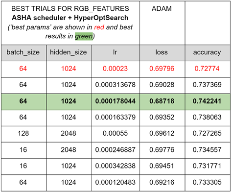
The last step to optimize results was changing from default Ray Tune search algorithm (random and grid search) to HyperOptSearch. This algorithm uses the Tree-structured Parzen Estimators algorithm to perform a more efficient hyperparameter selection, and furthermore can leverage the best values found in the previous step (*) as input parameterization ('best params'). We expected that this allowed us to improve a bit more loss and accuracy. See Colab notebook here.
Tuning was run for 50 trials as well. Best trials are shown below:
So, the best final values found for hyperparameters were:
| Parameter | Final best value |
|---|---|
| Learning Rate | 0.000178044 |
| Batch Size | 64 |
| Hidden Layer size | 1024 |
obtaining
- Best trial final validation loss: 0.68718
- Best trial final validation accuracy: 0.742241
improving minimally (less than 2%) the previous results obtained with only ASHA scheduler.
We did finally a test using SGD optimizer but worst values were obtained.
Afterwards, a similar test was done with Flow features, showing a similar performance than for the RGB features, so we kept the same values obtained for RGB videos.
Unfortunately, we couldn't do the trials with the two-stream model since while running Ray Tune we discovered that a maximum 512MB filesize applied for total loaded pickle files during trial initialization, making it impossible to test it.
We tried to further increase the accuracy by performing some data augmentation on training data.
Since our dataset (Jester's subset) consists of videos in the form of frames, we could do this data augmentation either on the images or in the videos we make from them. We chose to apply it directly on the images as they are the primary source and it was easier to work with them; the script frameaug2video.py does the augmentation on the training images and creates the augmented videos from them.
We made use of the imgaug library to make this image transformations. This library allows to select and stack a wide range of them, including arithmetic (adding noise) and geometric changes, color, flips, pooling, resizing, etc. It was somehow complicated for us to chose a transformation (or a combination of them) since it had to be sufficiently relevant to improve our model but also enough careful to keep the gesture information. Besides of that, some transformations than can augment RGB videos don't change anything in the Optical Flow or even can ruin it.
So, keeping in mind our dataset and data treatment restrictions for our task:
- As we were working with Optical Flow, we could not apply blurs, adding noise or other image manipulation techniques that involved creating artificial motion as the resulting Optical Flow turned out to be completely useless.
- As we had direction-dependant gestures, horizontal flips had to be discarded.
We carried out a total of three trials in the search of the best transformations to be applied. Each of them includes the processes of data augmentation on training data: making augmented RGB videos from frames, extracting optical flow from them, extraction of augmented RGB and flow features and, finally, combination of previous features with the augmented ones in a single pickle file (one for RGB and another one for Flow) to feed the classifier network and train the model. Therefore, is a significant time-consuming task.
An scheme of the process is shown in the following picture:
To evaluate the trials we were using the final two-stream model and the script main_two_stream_OneCycleLR_save_best_model.ipynb with the following hyperparameters (those of the best model):
| Hyperparameter | Value |
|---|---|
| lr | 0.000178044 |
| batch_size | 64 |
| hidden_rgb | 1024 |
| hidden_flow | 1024 |
| dropout | 0.5 |
| epochs | 100 |
Make sure:
- That the pickle files fed to the model (the ones in /jester_dataset/features folder in Google Drive) correspond to the augmented dataset and
- That in /jester_dataset/csv folder there are the right files from csv_augm folder that can be found here inside jester_dataset.
In the first trial we applied a 15% zoom in the images, followed by random controlled changes in contrast, brightness, hue and saturation (the same for all the frames inside of a video).
As can be seen, overfitting occurs from epoch 48 approx. There isn’t any improvement due to data augmentation since validation loss is lower than the best values obtained previously, besides the fact that validation accuracy doesn't even reach 0.8.
As the first trial didn't improve the previous results, in the second one we tried another kind of transformations. We applied a 20% random translation in both directions in the images (the same for all the frames inside of a video).
Results are way better than those in previous trial. If we take a closer look at validation values:

We see that the model overfits above epoch 53 approx. At this time the validation accuracy reaches a peak value of 0.8325, which is a minor improvement over the previous best value obtained without augmentation that was 0.8312. However, it must be taken into account that, excluding this point, all the previous accuracy values were below 0.825.
Encouraged by the increase in accuracy in Trial II, we kept the same translation change that seemed to work in the right direction but adding a previous 15% zoom in the images. The results can be viewed below:
Once again overfitting is observed for epochs > 40 and accuracy doesn’t even reach 0.8 one more time. It seems that applying zoom isn’t suitable for augmenting our data.
A series of trials were carried out to have more data to train our network in the hope of obtaining a better global accuracy. Unfortunately, the obtained results did not show an improvement from the best model we already had, so further exploration of the technique was discarded.
Some of the reasons of why data augmentation haven't helped with our task could be:
- Not being able to fine-tune the last layers of the i3d_resnet50_v1_kinetics400 Mxnet model by unfreezing them, only the classifier could be trained. Thus, adding more training videos didn't result in a improvement because the classifier was already fitted for our task. That is also the reason why the augmented model presented overfitting over epoch 40 while the original one didn't.
- The pre-trained i3d_resnet50_v1_kinetics400 Mxnet model took already into account this sort of basic transformations to images (videos) in its ImageNet and Kinetics training, therefore feeding new similar ones didn't contribute to relevant information for our Deep Learning network.
- Or, perhaps, we just weren't able to find the right transformations to apply, and introducing this way new information to make a more robust network capable of better inferring.
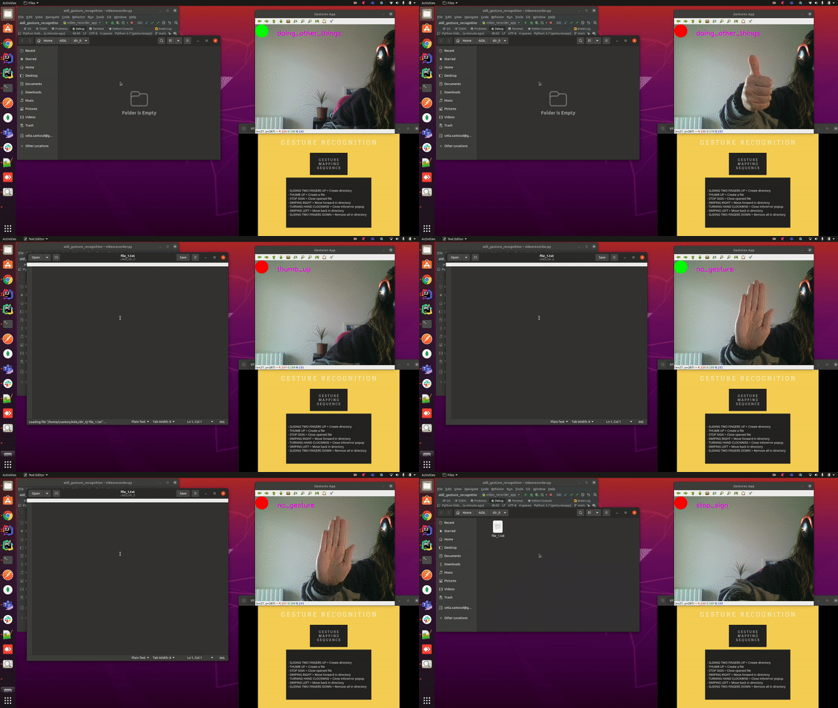
As stated in the introduction, our project goal was not only to train a working classifier but to use it to control a device. In our case, we decided to control our personal computer mapping some hand gestures to actions that will be displayed in a file window on a computer with a Linux OS GUI.
| Gesture | Action |
|---|---|
| Thumb Up | Create a file |
| Stop Sign | Close opened file |
| Sliding Two Fingers Up | Create directory |
| Sliding Two Fingers Down | Remove all in directory |
| Swiping Left | Move to previous directory |
| Swiping Right | Move to forward directory |
| Turning Hand Clockwise | Close info/error popup |
Note that the classes No Gesture and Doing Other Things are obviously not mapped to any action.
As we have commented, this project is made up of two different modules, which work in consonance using the client-server paradigm.
- video_processor (This module)
- video_capture. Added as a submodule in this repository.
In this way, the tasks are shared between the resource provider or server (video_processor) and the client (video_capture), which makes requests to the server and waits for its response to decide what action to take.
This architecture allows that, if a user does not have GPU resources on their local computer, they can deploy the server (video_processor) on another platform or resource provider (in our case we have used a GCP GPU), and the client application (video_capture) in charge of using the computer camera to record the videos on the local computer.
Thus, the way the whole system works is as follows: videos are captured in our computer, sent to the Cloud where they are processed and classified, and then a response is returned and the computer performs the action contained on it.
To manage the messages sent between server and client, we use Remote Procedure Calls (RPC) which is a protocol that a computer uses to execute code on another remote machine without having to worry about communications between both of them. This is handled by the open source AMQP message Broker RabbitMQ.
The following image shows all the modules of the complete project and how the management of the messages is done by the broker.
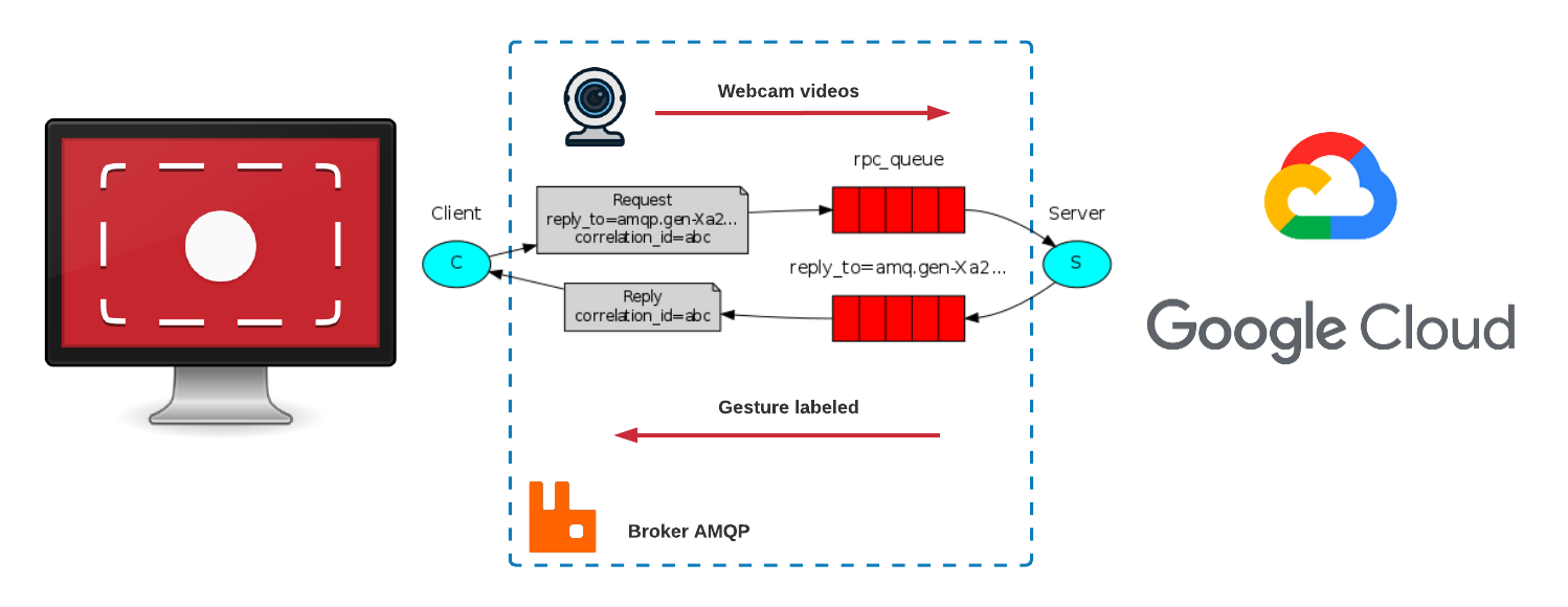
To be consistent with the training data, the videos processed will be 3 seconds long, captured at 12 fps and of the typical Jestser Dataset size [170,100]. As once we send the message containing a video it waits for a response, there is approximately one second (the time it usually takes to process the video) where the webcam is not recording. In order to help the user with the gesture timing, we added a dot on the screen that will be green if the camera is recording, and red if not.
Once the videos are received on Google Cloud, their Optical Flow is computed and the respective features are extracted from them, which go through the classification network. Then, a message is sent to our computer containing the class with the highest probability as well as the probability value.
When the response message is received, if the probability value exceeds a certain threshold the corresponding action is executed. We use thresholds because as we are performing real actions on the computer, we want the model to be confident enough on the predictions.
A full demo of all gestures with the corresponding Linux actions can be seen here.
In order to download the Jester Dataset, go to its official web page and then go to download section.
Notice that it is required to create an account in order to be able to download the dataset.
Download all the files with name 20bn-jester-v1-xx where xx is a number from 00 to 22 in your computer, all in the same directory. Once you have the 23 files downloaded, extract using:
$ cat 20bn-jester-v1-?? | tar zx This command will create a folder in your computer named 20bn-jester-v1 with 148.092 folders inside, and each one containing an average of 35 images in .jpg format (video frames of 3 seconds).
Create a new folder in your computer with name csvs and download the following files from the same Jestes Dataset downloads page:
train.csv
validation.csv
test.csv
labels.csv
Now you have the entire dataset ready and we need to clean it in order to get rid of the classes that are out of the scope of this project (Remember, we are only going to keep and train 9 classes of the 27 the dataset provides).
CLEAN VIDEOS
Now, we need to separate and remove all the videos from the classes that we won't use. We have 3 sets: train, validation and test. As the test set is not tagged and labeled, we cannot easily discard the videos from the classes we do not use. So the first step is to remove all the videos from unused classes of the traning and validation set, and separate the test ones.
To do so, we will use the file delete_unuseful_classes.py.
Change variables abs_path_to_csvs and abs_path_to_dataset in order to add the absolute path to your csvs folder and 20bn-jester-v1 respectively.
This script will only keep the train and validation videos of our useful 9 classes, and move to a new folder named test_set all the videos from the test set. This folder will be created in abs_path_to_dataset_folder you defined.
CLEAN CSVS
Delete all rows of the downloaded csvs to keep only the useful ones. We will use the file delete_unuseful_classes_csvs.py. To do so, replace the path_to_csvs_folder variable with the absolute path to your downloaded csvs folder. This script will create a new folder at the same folder level with name clean_csvs with the csv files filtered in order to only keep the labels of the useful classes.
At that point, we have a bunch of folders with .jpg frames inside it. In order to perform all other actions (extract optical flow and extract features), we need to have them all in a video format. To do so, we will use the following script: frame2video.py. We have to indicate the folder where the dataset is stored in abs_path_to_dataset variable and run the script. THis script will create a new folder in the same directory called videos with the same structure than the 20bn-jester-v1 one. But inside each subfolder named with a number, it will contain a single file with extension .mp4 which is the video file that has merged the video gesture frames.
In order to get the apparent motion estimation of the objects we compute the optical flow of every video, and get a new one with its optical flow vectors of the moving objects during the video sequence. To do so, we will use the following script: optical_flow.py. We need to set the abs_path_to_videos_folder variable with the absolute path to our videos folder, and abs_path_to_folder_out variable, with the path to the directory where we want to store the optical flow videos.
Notice: The procedure to extract the features from the raw videos is the same as for the optical flow videos. In this example we explain how to do it with the raw videos.
STEP1:
Generate a videos.txt file that will contain the list of paths of all videos. To do so, place yourself outside your videos folder and run the following command:
$ find ./videos -name '*.mp4' > ./videos.txtSTEP2:
After that, download the script feat_extract.py and place it in the same directory where you have your videos folder. Create a new folder named raw_videos_features in the same directory and type the following command:
$ python ./feat_extract.py --data-list ./videos.txt --model i3d_resnet50_v1_kinetics400 --save-dir ./raw_videos_features --gpu-id -1 --log-name featuresRGB.log &This command will generate a .npy file for each video of the videos folder in the newly created raw_videos_features folder. Each .npy file contains a numpy array of size [1,2048], the video features.
Repeat this procedure with your optical flow videos in order to extract the optical flow features.
For reference purposes only, some processing times are shown:
create_video_no_augm: Average time for processing 10 videos (with no GPU @1):  5.0 s approx.
optical_flow_no_augm: Average time for processing 10 videos (with no GPU @1):  2.0 s approx.
create_video_augm#1:  Average time for processing 10 videos (with GPU @3):     2.0 s approx.
create_video_augm#2:  Average time for processing 10 videos (with GPU @3):     0.8 s approx.
create_video_augm#3:  Average time for processing 10 videos (with GPU @3):     1.1 s approx.
optical_flow_augm:    Average time for processing 10 videos (with GPU @3): 1.4-2.0 s approx.
extract_features:     Average time for processing 10 videos (with GPU @3):     1.6 s approx  (*)
extract_features:     Average time for processing 10 videos (with no GPU @1):  5.0 s approx  (3x compared to *)
extract features:     Average time for processing 10 videos (with no GPU @3): 70.0 s approx (44x compared to *)

@1: GCP n1-standard-16 (16 vCPU, 60 GB mem)
@2: GCP n1-standard-4 (4 vCPU, 15 GB mem) + 1 x NVIDIA Tesla K80 GPU
@3: local x86 computer (8 CPU, 32 GB mem) + 1 x NVIDIA GeForce RTX 2060 GPU
The training was done mainly in Google Colab since it provides a convenient access to GPU, except for a part of the trials for hyperparameter tuning that were executed in a local machine due to known GPU usage limits established by Google in their free platform.
The training code needs access to some files that are located in a Google Drive's folder and are copied to Colab filesystem for the sake of improving access time to data.
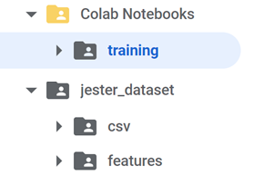
So it's necessary to create the following folder tree in your own Google Drive's root folder in order to you can execute the Jupyter notebooks scripts:
- Colab Notebooks: copy the notebooks in scripts/training folder from the repository and paste them in the training folder under your Colab Notebooks folder.
- jester_dataset: download from here and upload the contents under your Google Drive's jester_dataset folder according to the directory structure shown above.
- csv folder: contains the csv files with labels, and labeled training and validation data
- features folder: contains the RGB and flow features (extracted using the Gluon pre-trained model from the videos made from Jester Dataset) as pickle files
At this time you can already run the scripts used in training phase. They make use of GPU to accelerate training, so make sure you have this option on on Google Colab. To enable GPU in your notebook, select the following menu options:
Runtime / Change runtime type
and in Hardware accelerator select GPU.
As said above, these Python scripts use Jupyter notebook format and are as follows:
| File | Description |
|---|---|
| dataset.ipynb | Contains dataset class. Used by main* |
| models.ipynb | Contains models class. Used by main* |
| main.ipynb | Basic training (one stream, first & second approaches) |
| main_tune_ASHA.ipynb | Hyperparameter tuning with ray.Tune and ASHA scheduler (one stream, first & second approaches) |
| main_tune_ASHA+HYPEROPT.ipynb | Hyperparameter tuning with ray.Tune, ASHA scheduler and HyperOptSearch (one stream, first & second approaches) |
| main_two_stream.ipynb | Basic training (two-stream, third approach) |
| main_two_stream_OneCycleLR.ipynb | Training with OneCycleLR scheduler (two-stream, third approach) |
| main_two_stream_OneCycleLR_save_best_model.ipynb | Training with OneCycleLR scheduler (two-stream, third approach), saves best accuracy model parameters. Final model parameters are extracted with this code |
Before continuing, make sure you have Python installed and available from your command line. You can check this by simply running:
#!/bin/bash
$ python --version
Your output should look similar to: 3.8.2.
If you do not have Python, please install the latest 3.8 version from python.org.
Make sure you have docker installed in your computer by typing:
$ docker -vIf installed, you should get an output similar to: Docker version 20.10.3. If you do not have Docker, install the latest version from its official site: https://docs.docker.com/get-docker/
Make sure you have docker-compose installed in your computer by typing:
$ docker-compose -vIf installed, you should get an output similar to: docker-compose version 1.27.4. If you do not have docker-compose, install the latest version from its official site: https://docs.docker.com/compose/install/
To test your installation, in your terminal window or Anaconda Prompt, run the command:
$ conda listAnd you should obtain the list of packages installed in your base environment.
Notice: This repository has been designed in order to allow being executed with two different environments. If you have a GPU in your computer, make use of the file "environment_gpu.yml" during the next section, in case you only have CPU, use the file "environment.yml" to prepare your environment.
Execute:
$ conda env create -f environment_gpu.ymlThis will generate the videoprocgpu environment with all the required tools and packages installed.
Once your environment had been created, activate it by typing:
$ conda activate videoprocgpuCreate a folder with name /env inside the video_processor root directory folder and then, create a .env file inside it.
Copy the following code to your .env file:
RABBIT_USER="..."
RABBIT_PW="..."
RABBIT_HOST="..."
RABBIT_PORT="..."
VIDEOS_OUT_PATH="..."
MODEL_DIR="..."
GPU="..."
Replace the dots in your .env file with the following information:
- RABBIT_USER: Default rabbit username.
- RABBIT_PW: Default rabbit user password.
- RABBIT_HOST: The IP or domain name where your rabbit service is hosted.
- RABBIT_PORT: Default port of your rabbit service.
- VIDEOS_OUT_PATH: Absolute path to the folder where you want to store your real time capturing videos.
- MODEL_DIR: Absolute path to the
./modelsfolder. By default this directory is placed at the root of this repository. - GPU: This field should be set to
Truein case you are using one GPU andFalsein case you are not.
Activate the project service dependencies by starting a rabbitmq container. Go to the /deployment folder and edit the docker-compose.yml file in order to add your user and password credentials.
- ${RABBIT_USER}: Replace by your rabbit default user name.
- ${RABBIT_PW}: Replace by your rabbit default password.
When your credentials had been set, from the same directory type:
$ docker-compose up rabbitmqFinally, to start the video_processor app, place yourself in the repository root dir and type:
$ python3 app/app.pyNow, the video processor app will be running as a process in your terminal and the server will be waiting for requests. You will see a log in your command line like the following:
[X] Start Consuming:
Please, refer to the video_capture repository README in order to get the instructions to run the client app.


