
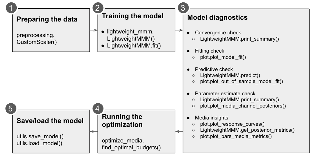
LightweightMMM 🦇 is a lightweight Bayesian Marketing Mix Modeling (MMM) library that allows users to easily train MMMs and obtain channel attribution information. The library also includes capabilities for optimizing media allocation as well as plotting common graphs in the field.
It is built in python3 and makes use of Numpyro and JAX.
- Easily train your marketing mix model.
- Evaluate your model.
- Learn about your media attribution and ROI per media channel.
- Optimize your budget allocation.
- Scale you data for training.
Some marketing practitioners pay attention to Marketing Mix Modeling (MMM) because of a couple of reasons. Firstly, measurement based on aggregated data is not affected by the recent ecosystem changes (some related to privacy) happening in the attribution model. Secondly, advertisers and their marketing partners have the data science resources to consider in-house MMM capability to nurture their analytics capabilities and accumulate insights by themselves. Taking consideration of the emerging situations, an open-source MMM solution is launched.
For larger countries we recommend a geo-based model.
We estimate a model where we use sales revenue (y) as the KPI. All parameters
will be estimated simultaneously by using MCMC sampling. Prior distribution of
the parameters is preset. Users can change the prior distributions in model.py
file if necessary. However, this is not a straight forward way and we recommend
you to keep this.

Seasonality is a latent sinusoidal parameter with a repeating pattern. Default degrees of the seasonality is 2.
Media parameter beta_m is informed by costs. It uses a HalfNormal distribution
and the scale of the distribution is the total cost of each media channel.
We have three different versions of the MMM with different lagging and saturation and we recommend you compare all three models. The Adstock and carryover models have an exponent for diminishing returns. The Hill functions covers that functionality for the Hill-Adstock model.
- Adstock: Applies an infinite lag that decreases its weight as time passes.
- Hill-Adstock: Applies a sigmoid like function for diminishing returns to the output of the adstock function.
- Carryover: Applies a causal convolution giving more weight to the near values than distant ones.
Options for lagging and saturation are as follows. Users can specify the option with model_name parameter in LightweightMMM class.

LightweightMMM is a class defined by lightweight_mmm.py.
The recommended way of installing lightweight_mmm is through PyPi:
pip install lightweight_mmm
If you want to use the most recent and slightly less stable version you can install it from github:
pip install --upgrade git+https://github.com/google/lightweight_mmm.git
Here we use simulated data but it is assumed you have your data cleaned at this point. The necessary data will be:
- Media data: Containing the metric per channel and time span (eg. impressions per week). Media values must not contain negative values.
- Extra features: Any other features that one might want to add to the analysis. These features need to be known ahead of time for optimization or you would need another model to estimate them.
- Target: Target KPI for the model to predict. For example, revenue amount, number of app installs. This will also be the metric optimized during the optimization phase.
- Costs: The average cost per media unit per channel.
# Let's assume we have the following datasets with the following shapes (we use
the `simulate_dummy_data` function in utils for this example):
media_data, extra_features, target, costs = utils.simulate_dummy_data(
    data_size=160,
    n_media_channels=3,
    n_extra_features=2,
    geos=5) # Or geos=1 for national model
Scaling is a bit of an art, Bayesian techniques work well if the input data is small scale. We should not center variables at 0. Sales and media should have a lower bound of 0.
ycan be scaled asy / jnp.mean(y).mediacan be scaled asX_m / jnp.mean(X_m, axis=0), which means the new column mean will be 1.
We provide a CustomScaler which can apply multiplications and division scaling
in case the wider used scalers don't fit your use case. Scale your data
accordingly before fitting the model.
Below is an example of usage of this CustomScaler:
# Simple split of the data based on time.
split_point = data_size - data_size // 10
media_data_train = media_data[:split_point, :]
target_train = target[:split_point]
extra_features_train = extra_features[:split_point, :]
extra_features_test = extra_features[split_point:, :]

# Scale data
media_scaler = preprocessing.CustomScaler(divide_operation=jnp.mean)
extra_features_scaler = preprocessing.CustomScaler(divide_operation=jnp.mean)
target_scaler = preprocessing.CustomScaler(
    divide_operation=jnp.mean)
# scale cost up by N since fit() will divide it by number of weeks
cost_scaler = preprocessing.CustomScaler(divide_operation=jnp.mean)

media_data_train = media_scaler.fit_transform(media_data_train)
extra_features_train = extra_features_scaler.fit_transform(
    extra_features_train)
target_train = target_scaler.fit_transform(target_train)
costs = cost_scaler.fit_transform(unscaled_costs)
In case you have a variable that has a lot of 0s you can also scale by the mean
of non zero values. For instance you can use a lambda function to do this:
lambda x: jnp.mean(x[x > 0]). The same applies for cost scaling.
The model requires the media data, the extra features, the costs of each media unit per channel and the target. You can also pass how many samples you would like to use as well as the number of chains.
For running multiple chains in parallel the user would need to set
numpyro.set_host_device_count to either the number of chains or the number of
CPUs available.
See an example below:
# Fit model.
mmm = lightweight_mmm.LightweightMMM()
mmm.fit(media=media_data,
        extra_features=extra_features,
        total_costs=costs,
        target=target,
        number_warmup=1000,
        number_samples=1000,
        number_chains=2)
You can switch between daily and weekly data by enabling
weekday_seasonality=True and seasonality_frequency=365 or
weekday_seasonality=False and seasonality_frequency=52 (default). In case
of daily data we have two types of seasonality: discrete weekday and smooth
annual.
Users can check convergence metrics of the parameters as follows:
mmm.print_summary()
The rule of thumb is that r_hat values for all parameters are less than 1.1.
Users can check fitting between true KPI and predicted KPI by:
plot.plot_model_fit(media_mix_model=mmm, target_scaler=target_scaler)
If target_scaler used for preprocessing.CustomScaler() is given, the target
would be unscaled. Bayesian R-squared and MAPE are shown in the chart.
Users can get the prediction for the test data by:
prediction = mmm.predict(
    media=media_data_test,
    extra_features=extra_data_test,
    target_scaler=target_scaler
)
Returned prediction are distributions; if point estimates are desired, users
can calculate those based on the given distribution. For example, if data_size
of the test data is 20, number_samples is 1000 and number_of_chains is 2,
mmm.predict returns 2000 sets of predictions with 20 data points. Users can
compare the distributions with the true value of the test data and calculate
the metrics such as mean and median.
Users can get detail of the parameter estimation by:
mmm.print_summary()
The above returns the mean, standard deviation, median and the credible interval for each parameter. The distribution charts are provided by:
plot.plot_media_channel_posteriors(media_mix_model=mmm, channel_names=media_names)
channel_names specifies media names in each chart.
Response curves are provided as follows:
plot.plot_response_curves(media_mix_model=mmm, media_scaler=media_scaler, target_scaler=target_scaler)
If media_scaler and target_scaler used for preprocessing.CustomScaler() are given, both the media and target values would be unscaled.
To extract the media effectiveness and ROI estimation, users can do the following:
media_effect_hat, roi_hat = mmm.get_posterior_metrics()
media_effect_hat is the media effectiveness estimation and roi_hat is the ROI estimation. Then users can visualize the distribution of the estimation as follows:
plot.plot_bars_media_metrics(metric=media_effect_hat, channel_names=media_names)
plot.plot_bars_media_metrics(metric=roi_hat, channel_names=media_names)
For optimization we will maximize the sales changing the media inputs such that the summed cost of the media is constant. We can also allow reasonable bounds on each media input (eg +- x%). We only optimise across channels and not over time. For running the optimization one needs the following main parameters:
n_time_periods: The number of time periods you want to simulate (eg. Optimize for the next 10 weeks if you trained a model on weekly data).- The model that was trained.
- The
budgetyou want to allocate for the nextn_time_periods. - The extra features used for training for the following
n_time_periods. - Price per media unit per channel.
media_gaprefers to the media data gap between the end of training data and the start of the out of sample media given. Eg. if 100 weeks of data were used for training and prediction starts 2 months after training data finished we need to provide the 8 weeks missing between the training data and the prediction data so data transformations (adstock, carryover, ...) can take place correctly.
See below and example of optimization:
# Run media optimization.
budget = 40 # your budget here
prices = np.array([0.1, 0.11, 0.12])
extra_features_test = extra_features_scaler.transform(extra_features_test)
solution = optimize_media.find_optimal_budgets(
    n_time_periods=extra_features_test.shape[0],
    media_mix_model=mmm,
    budget=budget,
    extra_features=extra_features_test,
    prices=prices)
Users can save and load the model as follows:
utils.save_model(mmm, file_path='file_path')
Users can specify file_path to save the model.
To load a saved MMM model:
utils.load_model(file_path: 'file_path')
While Lightweight MMM does not have features to apply a posterior distribution to
a new model training at this moment, users can adjust parameters of the prior
distributions in model.py and media_transforms.py when necessary. However,
this is not a straight forward way and we recommend you to keep this.
A model with 5 media variables and 1 other variable and 150 weeks, 1500 draws and 2 chains should take 6 mins per chain to estimate (on CPU machine).