A control systems design toolbox for Julia.
To install, in the Julia REPL:
using Pkg; Pkg.add("ControlSystems")ControlSystems have now been divided into two packages:
- ControlSystemsBase.jl lives in this same repository in the folder
lib/, and contains most of the original functionality of ControlSystems, except continuous-time simulation and root locus. - ControlSystems.jl internally uses and reexports ControlSystemsBase.jl and adds continuous-time simulation.
This is not a breaking change, users of ControlSystems.jl will have the same functionality now as before, but users who do not need continuous-time simulation (including simulation of delay systems and nonlinear systems) can use the considerably more lightweight ControlSystemsBase.jl package instead.
OrdinaryDiffEq.jl and DelayDiffEq.jl contributed the vast majority of both pre-compilation time and loading time of ControlSystems.jl, and workflows that do not require these packages were thus burdened by this overhead unnecessarily. If you do not need this, install and use ControlSystemsBase rather than ControlSystems (do not even install ControlSystems to avoid the pre-compilation time of OrdinaryDiffEq).
We still encourage advanced users to build a system image following the instructions in the documentation, but in the absence of such a system image, we now have the following timings:
julia> @time using ControlSystemsBase
1.70 secondsjulia> @time using ControlSystems
10.90 secondsNew feature: loopshapingPID
Release notes: https://github.com/JuliaControl/ControlSystems.jl/releases
Better support for static systems (using StaticArrays)
- Breaking: Frequency-responses have changed data layout to
ny×nu×nωfrom the previousnω×ny×nu. This is for performance reasons and to be consistent with time responses. This affects downstream functionsbodeandnyquistas well. - Breaking:
baltruncandbalrealnow return the diagonal of the Gramian as the second argument rather than the full matrix. - Breaking: The
pidconstructor no longer takes parameters as keyword arguments.pidhas also gotten some new features, the new signature ispid(P, I, D=0; form = :standard, Ts=nothing, Tf=nothing, state_space=false). This change affects downstream functions likeplacePI, loopshapingPI, pidplots. - Breaking: The semantics of broadcasted multiplication between two systems was previously inconsistent between
StateSpaceandTransferFunction. The new behavior is documented under Multiplying systems in the documentation.
All functions have docstrings, which can be viewed from the REPL, using for example ?tf .
A documentation website is available at http://juliacontrol.github.io/ControlSystems.jl/dev/ and an introductory video is available here.
Some of the available commands are:
ss, tf, zpk, delay
poles, tzeros, norm, hinfnorm, linfnorm, ctrb, obsv, gangoffour, margin, markovparam, damp, dampreport, zpkdata, dcgain, covar, gram, sigma, sisomargin
are, lyap, lqr, place, leadlink, laglink, leadlinkat, rstd, rstc, dab, balreal, baltrunc
pid, stabregionPID, loopshapingPI, pidplots, placePI
step, impulse, lsim, freqresp, evalfr, bode, nyquist
bodeplot, nyquistplot, sigmaplot, plot(lsim(...)), plot(step(...)), plot(impulse(...)), marginplot, gangoffourplot, pzmap, nicholsplot, pidplots, rlocus, leadlinkcurve
minreal, sminreal, c2d
This toolbox works similar to that of other major computer-aided control systems design (CACSD) toolboxes. Systems can be created in either a transfer function or a state space representation. These systems can then be combined into larger architectures, simulated in both time and frequency domain, and analyzed for stability/performance properties.
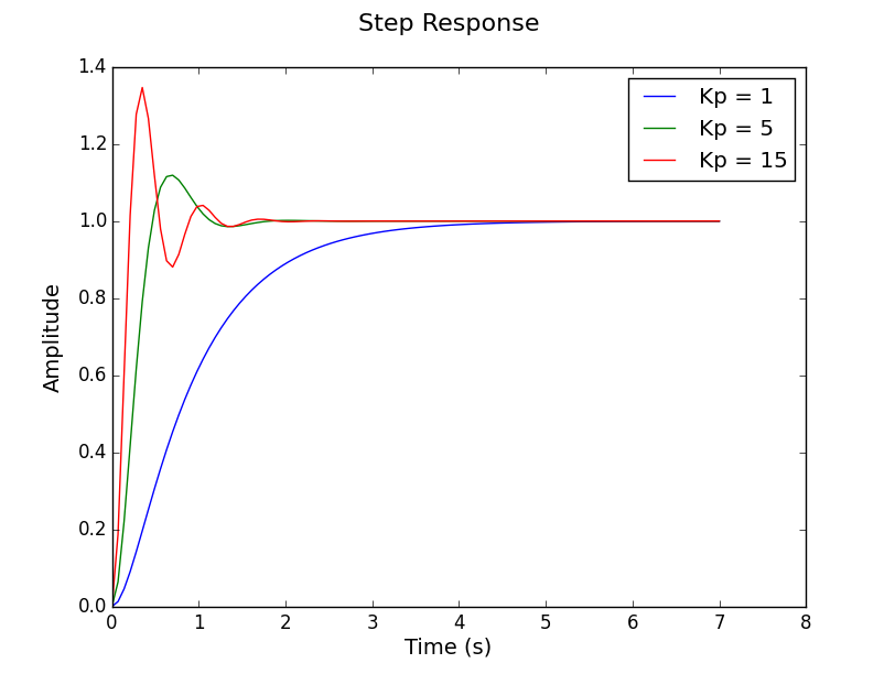
Here we create a simple position controller for an electric motor with an inertial load.
using ControlSystems

# Motor parameters
J = 2.0
b = 0.04
K = 1.0
R = 0.08
L = 1e-4

# Create the model transfer function
s = tf("s")
P = K/(s*((J*s + b)*(L*s + R) + K^2))
# This generates the system
# TransferFunction:
#                1.0
# ---------------------------------
# 0.0002s^3 + 0.160004s^2 + 1.0032s
#
#Continuous-time transfer function model

# Create an array of closed loop systems for different values of Kp
CLs = TransferFunction[kp*P/(1 + kp*P) for kp = [1, 5, 15]];

# Plot the step response of the controllers
# Any keyword arguments supported in Plots.jl can be supplied
using Plots
plot(step.(CLs, 5), label=["Kp = 1" "Kp = 5" "Kp = 15"])See the examples folder and ControlExamples.jl and several examples in the documentation.


