The dataset, a record of about 110,00 medical appointments in brazil focuses on whether a patient showed up for a scheduled appointment. The dataset contains 14 variables (columns) which are:
- PatientId - Identification of the patient
- AppointmentID - Identification of the appointment
- Gender - (M)ale or (F)emale
- ScheduledDay - The day the patient set up the appointment
- AppointmentDay - The day of the appointment
- Age - Age of the patient
- Neighbourhood - The location of the hospital.
- Scholarship - Whether or not the patient was enrolled in the Brazilian welfare program (0 = False, 1 = True)
- Hipertension - Whether or not the patient had Hypertension (0 = False, 1 = True)
- Diabetes - Was the patient diabetic? (0 = False, 1 = True)
- Alcoholism - Was the patient an alcoholic? (0 = False, 1 = True)
- Handcap - Was the patient handicapped? (0 = False, 1 = True)
- SMS_received - One (1) or more messages sent to the patient
- No-show - Did the patient not show up for the appointment? (No = Patient showed up, Yes = Patient did not)
More information about the dataset can be found here
What factors are important for us to know in order to predict if a patient will show up for their scheduled appointment? Specifically:
- Which gender is more likely to miss an appointment?
- Does the length of days between the schedule date and appointment date affect No-show?
- Does sending SMS reduce the number of No-shows?
- Are those in the Brazilian welfare program more likely to keep an appointment?
- Does the presence of any of the conditions (Hypertension, Diabetes, Alcoholism and Handicap) influence Noshow?
import pandas as pd
import numpy as np
import matplotlib.pyplot as plt
import seaborn as sns

%matplotlib inline
# Upgrade pandas to use dataframe.explode() function.
# !pip install --upgrade pandas==0.25.0# load the data
df = pd.read_csv('Database_No_show_appointments/noshowappointments-kagglev2-may-2016.csv')# let's see the first five rows
df.head().dataframe tbody tr th {
vertical-align: top;
}
.dataframe thead th {
text-align: right;
}
| PatientId | AppointmentID | Gender | ScheduledDay | AppointmentDay | Age | Neighbourhood | Scholarship | Hipertension | Diabetes | Alcoholism | Handcap | SMS_received | No-show | |
|---|---|---|---|---|---|---|---|---|---|---|---|---|---|---|
| 0 | 2.987250e+13 | 5642903 | F | 2016-04-29T18:38:08Z | 2016-04-29T00:00:00Z | 62 | JARDIM DA PENHA | 0 | 1 | 0 | 0 | 0 | 0 | No |
| 1 | 5.589978e+14 | 5642503 | M | 2016-04-29T16:08:27Z | 2016-04-29T00:00:00Z | 56 | JARDIM DA PENHA | 0 | 0 | 0 | 0 | 0 | 0 | No |
| 2 | 4.262962e+12 | 5642549 | F | 2016-04-29T16:19:04Z | 2016-04-29T00:00:00Z | 62 | MATA DA PRAIA | 0 | 0 | 0 | 0 | 0 | 0 | No |
| 3 | 8.679512e+11 | 5642828 | F | 2016-04-29T17:29:31Z | 2016-04-29T00:00:00Z | 8 | PONTAL DE CAMBURI | 0 | 0 | 0 | 0 | 0 | 0 | No |
| 4 | 8.841186e+12 | 5642494 | F | 2016-04-29T16:07:23Z | 2016-04-29T00:00:00Z | 56 | JARDIM DA PENHA | 0 | 1 | 1 | 0 | 0 | 0 | No |
# How many rows and columns does the data have?
df.shape
(110527, 14)
# inspect data types and look for instances of missing or possibly errant data.
df.info()
<class 'pandas.core.frame.DataFrame'>
RangeIndex: 110527 entries, 0 to 110526
Data columns (total 14 columns):
PatientId 110527 non-null float64
AppointmentID 110527 non-null int64
Gender 110527 non-null object
ScheduledDay 110527 non-null object
AppointmentDay 110527 non-null object
Age 110527 non-null int64
Neighbourhood 110527 non-null object
Scholarship 110527 non-null int64
Hipertension 110527 non-null int64
Diabetes 110527 non-null int64
Alcoholism 110527 non-null int64
Handcap 110527 non-null int64
SMS_received 110527 non-null int64
No-show 110527 non-null object
dtypes: float64(1), int64(8), object(5)
memory usage: 11.8+ MB
There are no missing data in any of the variables, however the ScheduledDay and AppointmentDay are not in the right types. Also Hipertension variable was wrongly spelt.
# Check the data for duplicates
df.duplicated().sum()
0
The following will be done to clean up the dataset for the sake of the intended analysis:
- Drop irrelevant variables (PatientId, AppointmentID, Neighbourhood)
- Rename variables for correctness (Hipertension, Handcap) and consistency (SMS_received, No-show)
- Convert ScheduledDay and AppointmentDay to the appropriate type (datetime)
- Keep only rows where the AppointmentDay is greater or same as the ScheduledDay
# Drop irrelevant columns/variables
df_clean = df.copy() # Make a copy of the original dataset for fallback or reference if neccessary

df_clean.drop(['PatientId', 'AppointmentID', 'Neighbourhood'], axis=1, inplace=True)

# view the columns left
df_clean.columns
Index(['Gender', 'ScheduledDay', 'AppointmentDay', 'Age', 'Scholarship',
'Hipertension', 'Diabetes', 'Alcoholism', 'Handcap', 'SMS_received',
'No-show'],
dtype='object')
# Rename variables for correctness and consistency
columns={'Hipertension': 'Hypertension', 'Handcap': 'Handicap', 'SMS_received': 'SmsReceived', 'No-show': 'NoShow'}
df_clean.rename(columns=columns, inplace=True)

df_clean.head(2).dataframe tbody tr th {
vertical-align: top;
}
.dataframe thead th {
text-align: right;
}
| Gender | ScheduledDay | AppointmentDay | Age | Scholarship | Hypertension | Diabetes | Alcoholism | Handicap | SmsReceived | NoShow | |
|---|---|---|---|---|---|---|---|---|---|---|---|
| 0 | F | 2016-04-29T18:38:08Z | 2016-04-29T00:00:00Z | 62 | 0 | 1 | 0 | 0 | 0 | 0 | No |
| 1 | M | 2016-04-29T16:08:27Z | 2016-04-29T00:00:00Z | 56 | 0 | 0 | 0 | 0 | 0 | 0 | No |
# Convert ScheduledDay and AppointmentDay to the appropriate type (datetime)
df_clean.ScheduledDay = pd.to_datetime(df_clean.ScheduledDay)
df_clean.AppointmentDay = pd.to_datetime(df_clean.AppointmentDay)

df_clean.info()
<class 'pandas.core.frame.DataFrame'>
RangeIndex: 110527 entries, 0 to 110526
Data columns (total 11 columns):
Gender 110527 non-null object
ScheduledDay 110527 non-null datetime64[ns]
AppointmentDay 110527 non-null datetime64[ns]
Age 110527 non-null int64
Scholarship 110527 non-null int64
Hypertension 110527 non-null int64
Diabetes 110527 non-null int64
Alcoholism 110527 non-null int64
Handicap 110527 non-null int64
SmsReceived 110527 non-null int64
NoShow 110527 non-null object
dtypes: datetime64[ns](2), int64(7), object(2)
memory usage: 9.3+ MB
# Keep only rows where AppointmentDay >= ScheduledDay
df_clean['ActualDateTimeDifference'] = df_clean.AppointmentDay - df_clean.ScheduledDay

# calculate the length of days (appointment day inclusive) from scheduled date
df_clean['LenDays'] = df_clean['ActualDateTimeDifference'] .dt.days + 1

df_clean[['ScheduledDay', 'AppointmentDay', 'ActualDateTimeDifference', 'LenDays', 'NoShow']].head(10).dataframe tbody tr th {
vertical-align: top;
}
.dataframe thead th {
text-align: right;
}
| ScheduledDay | AppointmentDay | ActualDateTimeDifference | LenDays | NoShow | |
|---|---|---|---|---|---|
| 0 | 2016-04-29 18:38:08 | 2016-04-29 | -1 days +05:21:52 | 0 | No |
| 1 | 2016-04-29 16:08:27 | 2016-04-29 | -1 days +07:51:33 | 0 | No |
| 2 | 2016-04-29 16:19:04 | 2016-04-29 | -1 days +07:40:56 | 0 | No |
| 3 | 2016-04-29 17:29:31 | 2016-04-29 | -1 days +06:30:29 | 0 | No |
| 4 | 2016-04-29 16:07:23 | 2016-04-29 | -1 days +07:52:37 | 0 | No |
| 5 | 2016-04-27 08:36:51 | 2016-04-29 | 1 days 15:23:09 | 2 | No |
| 6 | 2016-04-27 15:05:12 | 2016-04-29 | 1 days 08:54:48 | 2 | Yes |
| 7 | 2016-04-27 15:39:58 | 2016-04-29 | 1 days 08:20:02 | 2 | Yes |
| 8 | 2016-04-29 08:02:16 | 2016-04-29 | -1 days +15:57:44 | 0 | No |
| 9 | 2016-04-27 12:48:25 | 2016-04-29 | 1 days 11:11:35 | 2 | No |
df_clean.LenDays.describe()count 110527.000000
mean 10.183702
std 15.254996
min -6.000000
25% 0.000000
50% 4.000000
75% 15.000000
max 179.000000
Name: LenDays, dtype: float64
Wait!, we have appointments (e.g. -6 days) before schedule?. The above table shows us that days with values of 0 are actually appointments scheduled for the same day. We remove the row(s) with LenDays < 0.
# get the indices of rows we want to drop
indices = df_clean[df_clean.LenDays < 0].index

# remove the rows
df_clean.drop(indices, inplace=True)

df_clean.LenDays.describe()
count 110522.000000
mean 10.184253
std 15.255115
min 0.000000
25% 0.000000
50% 4.000000
75% 15.000000
max 179.000000
Name: LenDays, dtype: float64
# Determine the proportions of males and females
df_clean.Gender.value_counts(normalize=True)
F 0.649979
M 0.350021
Name: Gender, dtype: float64
65% of the patients were females while the rest 35% were males
def create_grouped_data(key):
    """
    Create a pandas grouped data with the provided key
    Args:
        key (str) - The key provided to the pandas DataFrame groupby method
    Returns:
        A pandas grouped data
    """
    return df_clean.groupby(key).NoShow.value_counts(normalize=True) * 100


gender_noshow = create_grouped_data('Gender')
def create_side_by_side_barchart(grouped_data, keys, labels=None, colors=('b', 'g'),
title='', ylab='Proportion(%)', xlab='No Show'):
"""
A helper function that creates a side by side (dodged) bar chart
Args:
grouped_data (pandas.core.series.Series) - The data created by pandas DataFrame groupby method
keys (iterable) - A list or tuple of category or levels of the variable passed to the groupby method
labels (iterable) - labels to use as the plot legend
ylab (str) - Y-axis label of the plot
xlab (str) - X-axis label of the plot
Returns:
None
"""
index = np.arange(grouped_data[keys[0]].count())
width = 0.35
if labels is None:
labels = keys
plt.bar(index, grouped_data[keys[0]], width, color=colors[0], label=labels[0])
plt.bar(index + width, grouped_data[keys[1]], width, color=colors[1], label=labels[1])
plt.ylabel(ylab)
plt.xlabel(xlab)
plt.title(title)
plt.xticks(index + width / 2, ['No', 'Yes'] * 2) # add xtick labels
# # legend
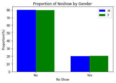
plt.legend();create_side_by_side_barchart(gender_noshow, keys=('M', 'F'), title='Proportion of Noshow by Gender')The same proportion (approx. 20%) of males and females did not show up for the scheduled appointment. This implied that Noshow is not influenced by gender.
It is pertinent to note that taking the days component alone (LenDays) meant a loss of the time component. My interest here is the days difference so it suffices for this question.
# I intend to use LenDays as a categorical variable since Noshow is a categorical variable
# let's see the 128 unique days
print('The {} unique days are: '.format(df_clean.LenDays.nunique()))
df_clean.LenDays.unique()
The 129 unique days are:
array([ 0, 2, 3, 1, 4, 9, 29, 10, 23, 11, 18, 17, 14,
28, 24, 21, 15, 16, 22, 43, 30, 31, 42, 32, 56, 45,
46, 39, 37, 38, 44, 50, 60, 52, 53, 65, 67, 91, 66,
84, 78, 87, 115, 109, 63, 70, 72, 57, 58, 51, 59, 41,
49, 73, 64, 20, 33, 34, 6, 35, 36, 12, 13, 40, 47,
8, 5, 7, 25, 26, 48, 27, 19, 61, 55, 62, 176, 54,
77, 69, 83, 76, 89, 81, 103, 79, 68, 75, 85, 112, 80,
86, 98, 94, 142, 155, 162, 169, 104, 133, 125, 96, 88, 90,
151, 126, 127, 111, 119, 74, 71, 82, 108, 110, 102, 122, 101,
105, 92, 97, 93, 107, 95, 139, 132, 179, 117, 146, 123])
# Let's see the distribution of the length of days
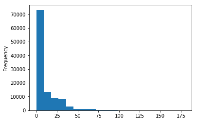
df_clean.LenDays.plot.hist(bins=20);
# A helper function to group the days
# We could further collapse the groups than what was done here
def group_days(days):
"""
Categorize number of days
Args:
days (int) - The days to group
Returns:
An integer between 0 and 8 (inclusive)
"""
if days == 0:
return 0
elif days <= 3:
return 1
elif days <= 7:
return 2
elif days <= 14:
return 3
elif days <= 30:
return 4
elif days <= 60:
return 5
elif days <= 90:
return 6
elif days <= 120:
return 7
elif days <= 150:
return 8
elif days <= 180:
return 9
df_clean['LenDaysGroup'] = df_clean.LenDays.map(group_days)
df_clean.LenDaysGroup.value_counts()0 38563
2 17510
4 17371
1 14675
3 12025
5 8283
6 1878
7 132
9 56
8 29
Name: LenDaysGroup, dtype: int64
days_group_noshow = create_grouped_data('LenDaysGroup')


noshow_yeses = [val for index, val in enumerate(days_group_noshow) if index % 2 != 0]
labels = ['Same Day', 'Within 3 Days', 'Within a Week', 'Within 2 Weeks', 'Within 1 Month', 'Within 2 Months', 'Within 3 Months',
                   'Within 4 Months', 'Within 5 Months', 'Within 6 Months']
index = np.arange(len(noshow_yeses))

# combine the index, yeses and labels so that it can be sorted accurately
data = list(zip(noshow_yeses, labels))

# sort the data by the yeses
data.sort(key=lambda x: x[0])

# transpose to the right shape for plotting: data[0] is now the index
data = list(zip(*data))

plt.figure(figsize=(8, 6))
plt.barh(index, data[0])
plt.xlabel('Proportion (%)')
plt.ylabel('Length of Days')
plt.title('Proportion of Noshow Based on Length of Days')
plt.yticks(index, data[1])
plt.show();
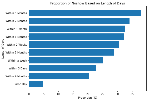
We see that less than 5% of same day (zero-day) appointments were not kept. The story is very different when the day of appointment is much later than the scheduled day.
Note that we could drill further into length of days with respect to gender and presence of disease or type of disease
# Find the proportion of those that were sent sms
df_clean.SmsReceived.value_counts(normalize=True)
0 0.67896
1 0.32104
Name: SmsReceived, dtype: float64
About 32% of the patients were sent 1 or more SMS
sms_noshow = create_grouped_data('SmsReceived')

labels = ('Received 0', 'Received 1 or more')
title = 'Proportion of Noshow Based on Number of SMS Received'
create_side_by_side_barchart(sms_noshow, keys=(0, 1), title=title, labels=labels)
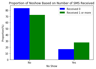
27.6% of those who received 1 or more SMS did not show up for their appointments while 16.7% of those who did not receive any sms did not show up for their appointments.
# How many people are in the welfare program?

# df_clean.Scholarship.value_counts(normalize=True) * 100
# Same as below

df_clean.Scholarship.mean() * 100 # We can do this because the column contains only 0s and 1s
9.8270027686795398
9.8% of the population were in the Brazilian welfare program
scholarship_noshow = create_grouped_data('Scholarship')
print(scholarship_noshow)
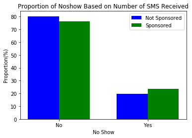
labels = ('Not Sponsored', 'Sponsored')
title = 'Proportion of Noshow Based on Number of SMS Received'

create_side_by_side_barchart(scholarship_noshow, keys=(0, 1), title=title, labels=labels)
Scholarship NoShow
0 No 80.196867
Yes 19.803133
1 No 76.263696
Yes 23.736304
Name: NoShow, dtype: float64
About 23.7% of those who were on welfare program missed their appointments while about 20% of those who were not did not keep their appointment.
has_any_condition = (df_clean.Hypertension == 1) | (df_clean.Diabetes == 1) | (df_clean.Alcoholism == 1)  | (df_clean.Handicap == 1)

df_condition = df_clean[has_any_condition]
df_no_condition = df_clean[has_any_condition == False]

print('{:.2f}% of the population had at least 1 of the listed conditions'.format(len(df_condition) / len(df_clean) * 100))
print('{:.2f}% of the population had none of the listed conditions'.format(len(df_no_condition) / len(df_clean) * 100))
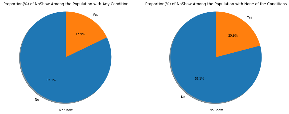
23.80% of the population had at least 1 of the listed conditions
76.20% of the population had none of the listed conditions
condition_noshow = df_condition.NoShow.value_counts(normalize=True) * 100
no_condition_noshow = df_no_condition.NoShow.value_counts(normalize=True) * 100

fig = plt.figure(figsize=(16, 6))
ax1, ax2 = fig.subplots(1, 2)

ax1.pie(condition_noshow, labels=condition_noshow.index, autopct='%1.1f%%',shadow=True, startangle=90)
ax1.axis('equal')  # Equal aspect ratio ensures that pie is drawn as a circle.
ax1.set_title('Proportion(%) of NoShow Among the Population with Any Condition')
ax1.set_xlabel("No Show")

ax2.pie(no_condition_noshow, labels=no_condition_noshow.index, autopct='%1.1f%%', shadow=True, startangle=90)
ax2.axis('equal')
ax2.set_title('Proportion(%) of NoShow Among the Population with None of the Conditions')
ax2.set_xlabel("No Show")

plt.show()
A larger proportion (20.9%) of those without any condition did not keep their appointments.
Firstly, it is pertinent to note that this analysis is tentative.
- Gender did not seem to influence the missing of hospital appointments (NoShow) among the population.
- Also, the length of days between scheduled date and appointment day seems to play a row on NoShow as 0 days (same-day) appointments were less missed.
- The reception of SMS seemed to influence NoShow. However, more insight could be gained if presence of disease or the length of days were considered along with receiving SMS.
- More proportion of those sponsored also missed their appointment relative to those who were not sponsored.
- Finally, more people without any condition (3% more than those with any condition) missed their appointment. Here also, we could probe further by checking which of the conditions (Hypertension or Diabetes or Alcoholism or Handicap) had more of NoShow.
The current analysis does not perform any hypothesis test which is necessary to provide concrete answers to the research questions. Secondly, statistically modelling (logistic regression) was not performed. This would give insights on the combination of factors that would predict NoShow.
# Create Html File Needed For Project Submission
from subprocess import call
call(['python', '-m', 'nbconvert', 'Investigate_a_Dataset.ipynb'])