This package may be used to assess statistical significance in hierarchical clustering. To assess significance in high-dimensional data, the approach assumes that a cluster may be well approximated by a single Gaussian (normal) distribution. Given the results of hierarchical clustering, the approach sequentially tests from the root node whether the data at each split/join correspond to one or more Gaussian distributions. The hypothesis test performed at each node is based on a Monte Carlo simulation procedure, and the family-wise error rate (FWER) is controlled across the dendrogram using a sequential testing procedure.
An illustration of the basic usage of the package's testing procedure is provided in the Testing section. Variations on the basic testing procedure are described in the associated subsections. Basic plotting procedures are described in the Plotting section.
To install sigclust2, which depends on packages in both CRAN and Bioconductor,
use the following call to the BiocManager package:
R> BiocManager::install("pkimes/sigclust2")
The package can then be loaded using the standard call to library.
suppressPackageStartupMessages(library("sigclust2"))While not necessary, installing the Rclusterpp package for faster clustering is recommended
when using sigclust2. Unforunately, the Rclusterpp package is no longer available on CRAN.
However, Rclusterpp can still be installed from the author's GitHub repo
with the following command from the devtools package (or
equivalently with a call to BiocManager::install again).
R> devtools::install_github("nolanlab/Rclusterpp")
For the following examples, we will use a simple toy example with 150 samples (n) with 100 measurements (p). The data are simulated from three Gaussian (normal) distributions.
set.seed(1508)
n1 <- 60; n2 <- 40; n3 <- 50; n <- n1 + n2 + n3
p <- 100
data <- matrix(rnorm(n*p), nrow=n, ncol=p)
data[, 1] <- data[, 1] + c(rep(2, n1), rep(-2, n2), rep(0, n3))
data[, 2] <- data[, 2] + c(rep(0, n1+n2), rep(sqrt(3)*3, n3))
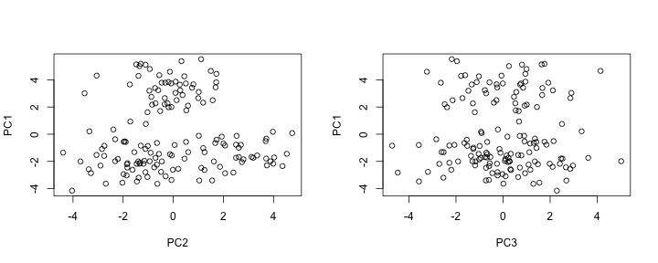
The separation of the three underlying distributions can be observed from a PCA (principal components analysis) scatterplot. While the separation is clear in the first 2 PCs, recall that the data actually exists in 100 dimensions.
data_pc <- prcomp(data)
par(mfrow=c(1, 2))
plot(data_pc$x[, 2], data_pc$x[, 1], xlab="PC2", ylab="PC1")
plot(data_pc$x[, 3], data_pc$x[, 1], xlab="PC3", ylab="PC1")
The SHC testing procedure is performed using the shc function. The function requires the following
three arguments:
x: the data as amatrixwith samples in rows,metric: the dissimilarity metric, andlinkage: the linkage function to be used for hierarchical clustering.
For reasons outlined in the corresponding paper (Kimes et al. 2017) relating to how
the method handles testing when n << p, we recommmend using "euclidean" as the metric,
and any of "ward.D2", "single", "average", "complete" as the linkage. If a custom
dissimilarity metric is desired, either of vecmet or matmet should be specified, as
described later in this section.
If metric functions which do not statisfy rotation invariance are desired,
e.g. one minus Pearson correlation ("cor") or L1 ("manhattan"),
null_alg = "2means" and ci = "2CI" should be specified. The null_alg and ci parameters
specify the algorithm for clustering and measure of "cluster strength" used to generate the null
distribution for assessing significance. Since the K-means algorithm (2means) optimizes
the 2-means CI (2CI), the resulting p-value will be conservative. However, since the hierarchical
algorithm is not rotation invariant, using null_alg = "hclust" or ci = "linkage" produces
unreliable results. An example for testing using Pearson correlation is given later in
this section.
For now, we just use the recommended and default parameters.
shc_result <- shc(data, metric="euclidean", linkage="ward.D2")The output is a S3 object of class shc, and a brief description of the analysis results can be
obtained by the summary function.
summary(shc_result)##
## shc object created using shc(..)
## --------------------------------
## Clustering Parameters:
## dissimilarity = euclidean
## linkage = ward.D2
## Testing Parameters:
## n_sim = 100
## icovest = 1
## ci = 2CI
## null_alg = hclust
## n_min = 10
## FWER control = FALSE
The analysis output can be accessed using the $ accessor. More details on the different entries
can be found in the documentation for the shc function.
names(shc_result)## [1] "in_mat" "in_args" "eigval_dat" "eigval_sim" "backvar"
## [6] "nd_type" "ci_dat" "ci_sim" "p_emp" "p_norm"
## [11] "idx_hc" "hc_dat"
The computed p-values are probably of greatest interest. Two p-values are computed as part of the
SHC testing procedure: (1) an empirical p-value (p_emp), and (2) a Gaussian approximate
p-value (p_norm). The p-values are computed based on comparing the observed strength of
clustering in the data against the expected strength of clustering under the null hypothesis
that the data from a single cluster. The null distribution is approximated using a
specified number of simulated datasets (n_sim = 100 default argument). p_emp is the empirical
p-value computed from the collection of simulated null datasets. p_norm is an approximation to
the empirical p-value which provides more continuous p-values. nd_type stores the results of the
test and takes values in: n_small, no_test, sig, not_sig, cutoff_skipped. With the default
implementation of shc using no FWER control, all nodes are either cutoff_skipped or n_small.
The p-values are reported for each of 149 (n-1) nodes along the hierarchical dendrogram.
The entries of p_emp and p_norm are ordered descending from the top of the dendrogram, with
the first entry corresponding to the very top (root) node of the tree.
data.frame(result = head(shc_result$nd_type, 5),
           round(head(shc_result$p_norm, 5), 5),
           round(head(shc_result$p_emp, 5), 5))
## result hclust_2CI hclust_2CI.1
## 1 cutoff_skipped 0.00000 0.00
## 2 cutoff_skipped 0.41475 0.37
## 3 cutoff_skipped 0.88019 0.90
## 4 cutoff_skipped 0.84834 0.85
## 5 cutoff_skipped 0.86693 0.88
In addition to values between 0 and 1, some p-values are reported as 2. These values correspond
to nodes which were not tested, either because of the implemented family-wise error rate (FWER)
controlling procedure (alpha) or the minimum tree size for testing (min_n).
Variations on the standard testing procedure are possible by changing the default parameters of
the call to shc(..).
The method also supports specifying your own metric function through the vecmet and matmet
parameters. Only one of vecmet and matmet should be specified. If either is specified, the
metric parameter will be ignored. The vecmet parameter should be passed a function which takes
two vectors as input and returns the dissimilarity between the two vectors. The matmet parameter
should be passed a function which takes a matrix as input and returns a dist object of
dissimilarities of the matrix rows.
The vecmet example is not actually run in this tutorial since it is incredibliy
computationally expensive. Internally, the function passed to vecmet is wrapped in the
following call to outer to compute dissimilarities between all rows of a matrix.
as.dist(outer(split(x, row(x)), split(x, row(x)), Vectorize(vecmet)))The following simple benchmarking example with cor illustrates the overhead for
using outer to call on a vector function rather than using an optimized matrix
dissimilarity function.
vfun <- function(x, y) {1 - cor(x, y)}
mfun1 <- function(x) {
    as.dist(outer(split(x, row(x)), split(x, row(x)),
                  Vectorize(vfun)))
}
mfun2 <- function(x) { as.dist(1 - cor(t(x))) }

system.time(mfun1(data))
## user system elapsed
## 1.884 0.053 1.997
system.time(mfun2(data))## user system elapsed
## 0.001 0.000 0.002
The first matrix correlation function, mfun1, is written it
would be processed if vfun were passed to shc as vecmet. The second funtion,
mfun2, is a function that could be passed to matmet. The performance difference is
clearly significant.
When specifying a custom dissimilarity function for shc, it is important to
remember that the function must be used to compute dissimilarity matrices n_sim times
for each node. In our toy example where n_sim = 100 and n = 150, this means
calling on the dissimilarity function >10,000 times.
Our custom function, mfun2 can be passed to shc through the matmet parameter.
shc_mfun2 <- shc(data, matmet=mfun2, linkage="average")

data.frame(result = head(shc_mfun2$nd_type),
           round(head(shc_mfun2$p_norm), 5),
           round(head(shc_mfun2$p_emp), 5))
## result hclust_2CI hclust_2CI.1
## 1 cutoff_skipped 0.99845 1.00
## 2 cutoff_skipped 0.63709 0.69
## 3 cutoff_skipped 0.24079 0.24
## 4 cutoff_skipped 0.94164 0.94
## 5 cutoff_skipped 0.94411 0.96
## 6 cutoff_skipped 0.99639 1.00
Since the toy dataset is simulated with all differentiating signal lying in the first two dimensions, Pearson correlation-based clustering does a poor job at distinguishing the clusters, and the resulting p-values show weak significance.
As a shortcut, without having to specify matmet, if testing using (1 - cor(x)) is desired,
the following specification can be used.
data_pearson <- shc(data, metric="cor", linkage="average", null_alg="2means")The result will be equivalent to apply the original sigclust hypothesis test described
in Liu et al. 2008 at each node along the dendrogram.
By default, p-values are calculated at all nodes along the dendrogram with at least n_min
observations (default n_min = 10). The package includes a FWER controlling procedure which
proceeds sequentially from the top node such that daughter nodes are only tested if
FWER-corrected significance was achieved at the parent node. To reduce the total number of tests
performed, set alpha to some value less than 1.
shc_fwer <- shc(data, metric="euclidean", linkage="ward.D2", alpha=0.05)The FWER is noted in the summary of the resulting shc object, and can be seen in the nd_type
attribute, where most tests are now labeled no_test (with p_norm and p_emp values of 2).
data.frame(result = head(shc_fwer$nd_type, 10),
           round(head(shc_fwer$p_norm, 10), 5),
           round(head(shc_fwer$p_emp, 10), 5))
## result hclust_2CI hclust_2CI.1
## 1 sig 0.00000 0.00
## 2 not_sig 0.36017 0.27
## 3 no_test 2.00000 2.00
## 4 not_sig 0.86606 0.88
## 5 no_test 2.00000 2.00
## 6 no_test 2.00000 2.00
## 7 no_test 2.00000 2.00
## 8 no_test 2.00000 2.00
## 9 no_test 2.00000 2.00
## 10 no_test 2.00000 2.00
By default, p_norm p-values are used to test for significance against the FWER cutoffs,
but p_emp can be used by specifying p_emp = TRUE.
The shc function allows for testing along the same dendrogram simultaneously using
different measures of strength of clustering.
For example, it is possible to simultaneously test the above example using both the 2-means cluster index and the linkage value as the measure of strength of clustering.
data_2tests <- shc(data, metric="euclidean", linkage="ward.D2",
                   ci=c("2CI", "linkage"),
                   null_alg=c("hclust", "hclust"))
round(head(data_2tests$p_norm), 5)
## hclust_2CI hclust_linkage
## [1,] 0.00001 0.00152
## [2,] 0.42544 0.97613
## [3,] 0.83015 0.99999
## [4,] 0.86116 1.00000
## [5,] 0.81640 1.00000
## [6,] 0.98948 1.00000
The results of clustering using hclust_2CI and hclust_linkage are reported in the columns
of the analysis results. The relative performance of a few of these different combinations are
described in the corresponding manuscript when using Ward's linkage clustering.
When alpha < 1 is specified, the additional ci_idx parameter specifies the index of the test
that should be used when trying to control the FWER.
While looking at the p-values is nice, plots are always nicer than numbers. A nice way to
see the results of the SHC procedure is simply to call plot on the shc class object
created using the shc(..) constructor.
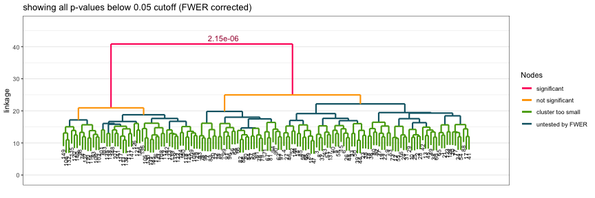
plot(shc_result, hang=.1)The resulting plot shows significant nodes and splits in red, as well as the corresponding p-values. Nodes which were not tested, as described earlier, are marked in either green or teal (blue).
Several types of diagnostic plots are implemented for the SHC method. These are available through the
diagnostic method. Since testing is performed separately at each node along the dendrogram, diagnostic
plots are also generated per-node. The set of nodes for which diagnostic plots should be generated
is specified with the K parameter. The default is to only generate plots for the root node, K = 1.
The method currently supports four types of diagnostic plots: background, qq, covest, pvalue.
The desired plot type is specified to the pty parameter as a vector of strings. To create all four
plots, simply specify all, which is also the default value.
If the length of K is greater than 1 or more than one plot type is specified, the method will
write files to a pdf file, fname.pdf, where fname is an input parameter that can be specifeid
by the user.
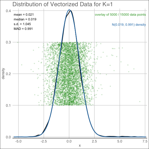
The background plot will return a jitter plot of the matrix entries, as well as a smooth kernel
density estimate and best-fit Gaussian approximation used in estimating the background
noise level.
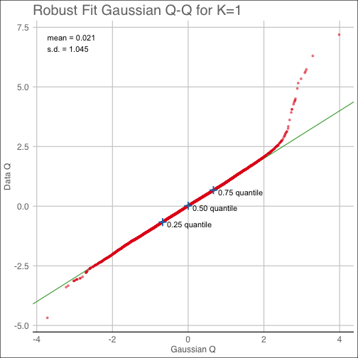
diagnostic(shc_result, K=1, pty='background')The qq plot provides the corresponding Quantile-Quantile plot from the background noise estimating
procedure.
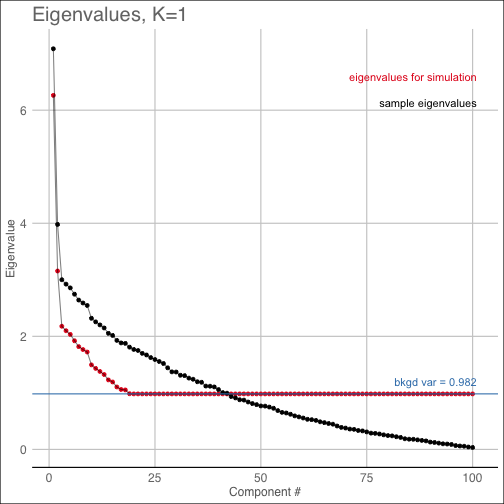
diagnostic(shc_result, K=1, pty='qq')The covest plot shows the estimated eigenvalues of the null Gaussian distribution along with the sample
eigenvalues of the original data matrix.
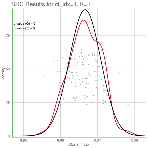
diagnostic(shc_result, K=1, pty='covest')The pvalue plot shows the cluster index for the original data along with the distribution of
simulated cluster indices used to determine the reported empirical (Q) p-value. Additionally, the
best-fit Gaussian approximation to the cluster index distirbution used to compute the Gaussian-approximate
(Z) p-value is overlaid in black.
diagnostic(shc_result, K=1, pty='pvalue')- Kimes PK, Liu Y, Hayes DN, and Marron JS. (2017). "Statistical significance for hierarchical clustering." Biometrics.
- Huang H, Liu Y, Yuan M, and Marron JS. (2015). "Statistical significance of clustering using soft thresholding." Journal of Computational and Graphical Statistics.
- Liu Y, Hayes DN, Nobel A, and Marron JS. (2008). "Statistical significance of clustering for high-dimension, low–sample size data." Journal of the American Statistical Association.
sessionInfo()## R version 3.5.0 (2018-04-23)
## Platform: x86_64-apple-darwin15.6.0 (64-bit)
## Running under: OS X El Capitan 10.11.6
##
## Matrix products: default
## BLAS/LAPACK: /usr/local/Cellar/openblas/0.2.20_2/lib/libopenblasp-r0.2.20.dylib
##
## locale:
## [1] en_US.UTF-8/en_US.UTF-8/en_US.UTF-8/C/en_US.UTF-8/en_US.UTF-8
##
## attached base packages:
## [1] stats graphics grDevices utils datasets methods base
##
## other attached packages:
## [1] sigclust2_1.2.4 bindrcpp_0.2.2 testthat_2.0.0 Rcpp_1.0.0
## [5] GGally_1.4.0 ggplot2_3.1.0
##
## loaded via a namespace (and not attached):
## [1] matrixStats_0.54.0 fs_1.2.6 usethis_1.4.0
## [4] fit.models_0.5-14 robust_0.4-18 devtools_2.0.0.9000
## [7] bit64_0.9-7 doParallel_1.0.14 RColorBrewer_1.1-2
## [10] rprojroot_1.3-2 dynamicTreeCut_1.63-1 tools_3.5.0
## [13] backports_1.1.2 R6_2.3.0 rpart_4.1-13
## [16] Hmisc_4.1-1 DBI_1.0.0 lazyeval_0.2.1
## [19] BiocGenerics_0.26.0 colorspace_1.3-2 nnet_7.3-12
## [22] withr_2.1.2 tidyselect_0.2.5 gridExtra_2.3
## [25] prettyunits_1.0.2 processx_3.2.0 preprocessCore_1.42.0
## [28] bit_1.1-14 compiler_3.5.0 WGCNA_1.66
## [31] cli_1.0.1 Biobase_2.40.0 htmlTable_1.12
## [34] ggdendro_0.1-20 desc_1.2.0 labeling_0.3
## [37] scales_1.0.0 checkmate_1.8.5 mvtnorm_1.0-8
## [40] DEoptimR_1.0-8 robustbase_0.93-3 callr_3.0.0
## [43] stringr_1.3.1 digest_0.6.18 foreign_0.8-71
## [46] rmarkdown_1.10 rrcov_1.4-4 base64enc_0.1-3
## [49] pkgconfig_2.0.2 htmltools_0.3.6 sessioninfo_1.1.1
## [52] highr_0.7 ggthemes_4.0.1 htmlwidgets_1.3
## [55] rlang_0.3.0.9000 rstudioapi_0.8 RSQLite_2.1.1
## [58] impute_1.54.0 bindr_0.1.1 acepack_1.4.1
## [61] dplyr_0.7.7 magrittr_1.5 GO.db_3.6.0
## [64] Formula_1.2-3 Matrix_1.2-14 munsell_0.5.0
## [67] S4Vectors_0.18.3 stringi_1.2.4 MASS_7.3-50
## [70] debugme_1.1.0 pkgbuild_1.0.2.9000 plyr_1.8.4
## [73] grid_3.5.0 blob_1.1.1 parallel_3.5.0
## [76] crayon_1.3.4 lattice_0.20-35 splines_3.5.0
## [79] knitr_1.20 ps_1.2.0 pillar_1.3.0
## [82] fastcluster_1.1.25 codetools_0.2-15 stats4_3.5.0
## [85] pkgload_1.0.1.9000 glue_1.3.0 evaluate_0.12
## [88] latticeExtra_0.6-28 data.table_1.11.8 remotes_2.0.1
## [91] foreach_1.4.4 gtable_0.2.0 purrr_0.2.5
## [94] reshape_0.8.7 assertthat_0.2.0 pcaPP_1.9-73
## [97] survival_2.42-6 tibble_1.4.2 iterators_1.0.10
## [100] AnnotationDbi_1.42.1
## [ reached getOption("max.print") -- omitted 3 entries ]
