This is material for the FOSS4G workshop held in Boston, MA in August 14, 2017.
Prepared by : Payam Tabrizian
Presented with: Anna Petrasova, Vaclav Petras, and Helena Mitasova
Tested and reviewed by: Garrett Millar
What if your geospatial data and simulations like flooding, fire-spread and viewshed computations are converted on-the-fly into realistic, interactive and immersive 3D worlds, without the need to deal with overly complicated or proprietary 3D modeling software? In this hands-on workshop we will explore how to automate importing and processing of various types of geospatial data (e.g., rasters, vectors) using Blender, an open-source 3D modeling and game engine software. We will start with a brief and focused introduction into Blender graphical user interface (GUI), Python API, as well as the GIS and Virtual reality addons. Once we import our GIS data into Blender, we will go over the techniques (both with GUI and command line) to increase the realism of our 3D world through applying textures, shading, and lighting. To make our work reusable for different projects, we will automate all importing and processing workflows using Python. Finally, we will show how to publish it online to share it with the world.
I. Intro
II. Basic components of blender interface
III. Editors
I. Setting up the scene
II. Georeferencing the blender Scene
III. Importing digital surface model
IV. Importing shapefile
V. Shading the scene
VI. 3D modeling made easy: scripting procedure
I. Intro to coupling with Modal Timer
II. Coupling with GIS data
I. Setting up the Blend4Web addon
II. Exporting blender scene to web format
| Section | Duration |
|---|---|
| Part 1 | 8:00- 9:45 |
| Break | 15 min |
| Part 2 | 10:00-11:00 |
| Part 3 | 11:00-11:30 |
| Part 4 | 11:30-12:00 |
Blender is an open-source 3D modeling, rendering and game engine software. You can create photorealistic scenes and life-like animations with it. The feature that makes Blender highly suitable for geospatial visualization is its capability to import various georeferenced data thanks to BlenderGIS addon. Almost every operation done in the blender interface, can be scripted in the Python scripting environment, allowing you to automate or batch process your 3D modeling workflow. Moreover, using Blend4Web or sketchfab addons, you would be able to publish your geospatial models online, so that everyone can interactively explore or download your work.
Learn more about Sketchfab
A sample geospatial model in Sketchfab
Blender has numerous components and features that, thanks to it open-source capabilities, are growing every day. Covering all aspects of the software itself require several lessons. The purpose of this section is to provide a brief introduction to Blender's graphical user interface and some of its features that are essential for working with geospatial data, and will be used throughout this tutorial. We will specifically introduce the following components: Areas, Editors, Tabs, Headers, Panels
- Browse the workshop materials folder, locate and open interface_introduction.blend
 Blender interface Blender interface |
|---|
Blender's application window can be flexibly arranged and divided up into a number of Areas. An area contains the workspace for a particular type of editor, like a 3D View Editor, or an Outliner. In figure above you can see the application window is divided into five areas, each assigned to an editor.
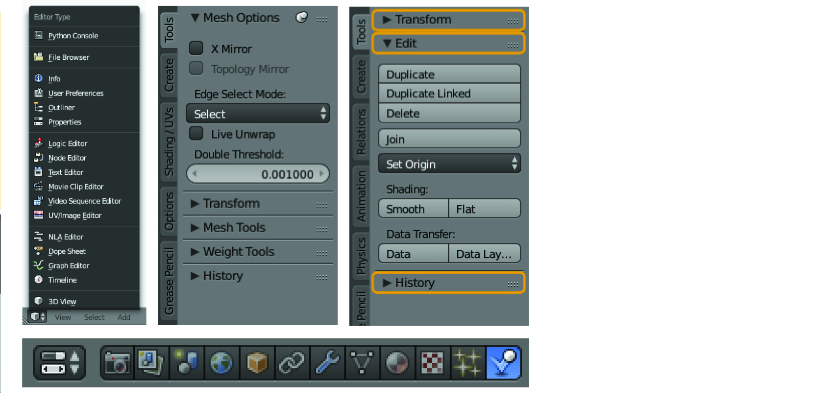
Editors are responsible for displaying and modifying different aspects of data. Imagine editors as full-fledge software each specialized for a specific tasks, like changing data properties, image editing, video editing, animation design, game design, and etc. You can assign an area to a specific editor using Editor Type selector , the first button at the left side of a header (figure below, left). Every area in Blender may contain any type of editor and it is also possible to open the same type multiple times.
Tabs are overlapping sections in the user-interface. Tabs can be vertical (Tool Shelf) or horizontal (Properties Editor, User Preferences).
Another common feature is the Header, that contain menus and commonly used tools specific to each editor. It has a small horizontal strip shape with a lighter gray background, which sits either at the top or bottom of the area.
Finally, the smallest organizational unit in the user interface is a Panel. You can usually collapse panels to hide their contents. They are used in the Properties Editor, but also for example in the Tool Shelf and the Properties region. In the image below on the right you can see three panels one of them is expanded and the rest are collapsed.
Above: Editor type selector (left), A Toolbar with tabs (middle), Toolbar Panels (right) Below: A Header with tabs
Now that you have some general ideas about the interface, we will review some of the commonly used editors.
The 3D View is the visual interface with the 3D data and scene with numerous functionalities for modeling, animation, texture painting, etc. Unlike the 2D environment of GIS software, where you can only navigate in x and y directions, 3D viewport allows full control over our viewing angle, depth, size, etc. You can press and hold down mouse scroll (or middle click) button to change the viewing angle (or orbiting around), shift and drag to pan, and roll to zoom back and forth.
Now note the panel on the left side of the region which is called Tool shelf and it has a variety of the tools for 3D editing. Newly installed addons also appear in this toolbar. Now notice the bottom Header. It includes menus for adding, editing objects as well as viewing and shading options.
 3D view header (retrieved from Blender manual) 3D view header (retrieved from Blender manual) |
|---|
Header's View menu allows you to select a specific viewpoint such as top, left or different perspectives. Each of these commands have a keyboard shortcut ,for example you can press numpad 3 (if you have a full keyboard) to switch to top view.
Add menu provides a list of different types of 2D and 3D object that can be added to a scene
In Object Interaction mode you can different aspect of data. In this tutorial we focus Object mode and Edit mode. Edit mode allows you to access more low-level structures of your object, like faces, and vertices. In the examples that we complete in this tutorial, we will use some of these options to refine the surface model. It is important to get familiar with the 3 core elements, Faces, Edges and Vertex. You can select these elements by clicking on their corresponding icons.
On the right side of the interaction mode, is the viewport Shading mode which you can use to choose the visualization and viewport rendering methods. Solid mode is the default mode and shows objects with solid faces, but without textures and shading. The Texture mode shows the object with textures. Material mode is the fast approximation of the complete material including texture and shading. Rendered mode enables real-time rendering, which computes the near-to-final product on-the-fly as you interact with the object (with accurate materials and lighting).
Objects are basically everything that you see in the 3D view. They include 3D objects, lights, cameras and more. You can select any object in the scene using the right-click. Selected objects are highlighted in orange. Use the 3 axes (i.e., handles) to move the object in your preferred direction. To select multiple objects, press and hold control key and right click on objects to add to your selection. To unselect hold shift and right-click on the object. You can move (grab) objects by pressing G, rotate them by pressing R, or scale them using S key. You can constrain any transformation to a specific axis by pressing x, y, z. You can delete the object by selecting it, pressing delete key and selecting ok.
As its name suggests, outliner lists and organizes the scene objects. From there you can set the hierarchy, visibility of the 3D objects or lock them if you need. You can also select and activate objects by clicking on their name in the list. Figure below shows Outliner editor that list three objects (Camera, Cube and Lamp) and the Lamp object is selected.
The Python console is a useful editor for testing and executing short commands, which then can be integrated in larger workflows. The Blender modeling and gaming modules are already loaded in python console so you can you can test your code snippets without extra effort of calling the modules.
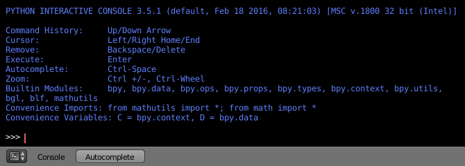 Python console (retrieved from Blender manual) |
|---|
Example 1. Simple object operation using python console.
- Call Cube object and print its location
- Copy and paste the individual command lines in the console and press enter
cubeObj = bpy.data.objects['Cube']
print (cubeObj.location)- Move cube object to location x = 0 , y = 2 , z = 3
cubeObj.location = (0, 2, 3)- Move cube object 5 units in positive X direction
cubeObj.location [0] += 5- Select and delete cube object
## Unselect everything in the scene
bpy.ops.object.select_all(action='DESELECT')
cubeObj.select = True
bpy.ops.object.delete()
Text editor allows you to edit your python script and run it inside Blender. By pressing the + icon you can start a new file and click on Run Script to execute your code. You need to call modeling and gaming modules in text editor.
 Text Editor |
|---|
Example 2. Batch processing simple object operations using text editor
- Create a matrix of 20 by 20 Cubes with varied size and location.
- In the text editor click on the + icon to create a new textfile
- Copy and paste the snippet below and click on Run script button
- The results should look like the figure below
import bpy
for x in range(20):
for y in range(20):
bpy.ops.mesh.primitive_cube_add(radius = .1 + (x*y*.0005), location=(x, y, (x*y*.02)))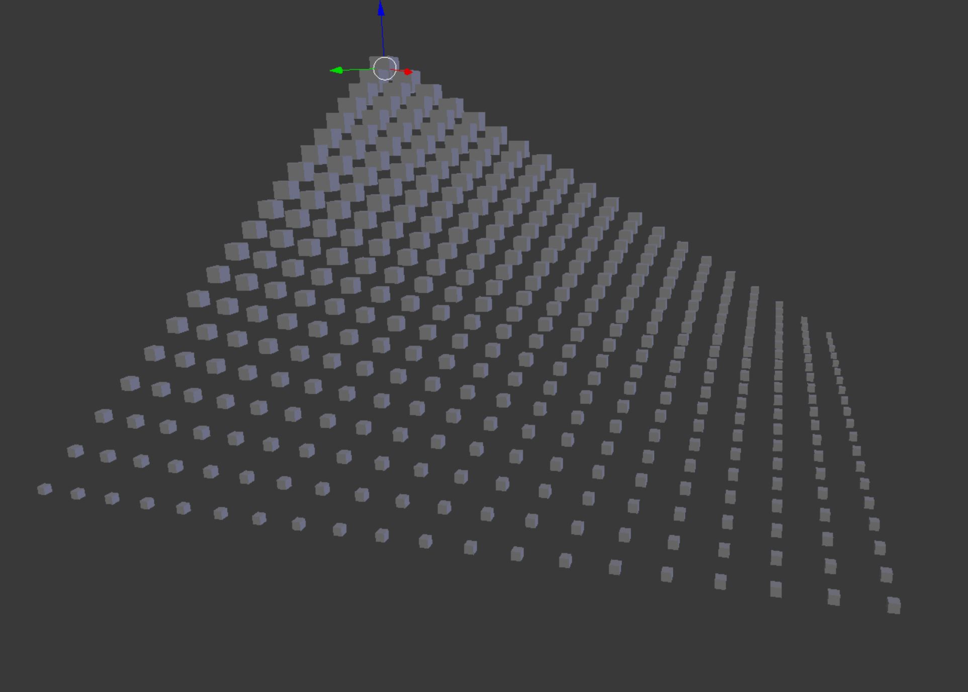 Cube matrix |
 Monkey and plane |
|---|
- Delete all cube objects, add a Monkey object, and add a Plane object
- Open a new text window or delete the contents of existing ones (select content with
ctrl + Aand pressdel)
- Open a new text window or delete the contents of existing ones (select content with
import bpy

# unselect object
bpy.ops.object.select_all(action='DESELECT')
## delete all object that have cube in their name ##
for object in bpy.data.objects:
    if "Cube" in object.name:
        object.select = True
        bpy.ops.object.delete()
## add monkey object
bpy.ops.mesh.primitive_monkey_add(location=(0, 0, 0), radius = 3)
## add plane object
bpy.ops.mesh.primitive_plane_add(location=(0, 0, -3), radius = 10)
Properties editor allows you to modify the properties of the scene, rendering setting, transforming objects or changing their material or texture properties. The components that we will work with in the following examples are Object, Material and Texture properties.
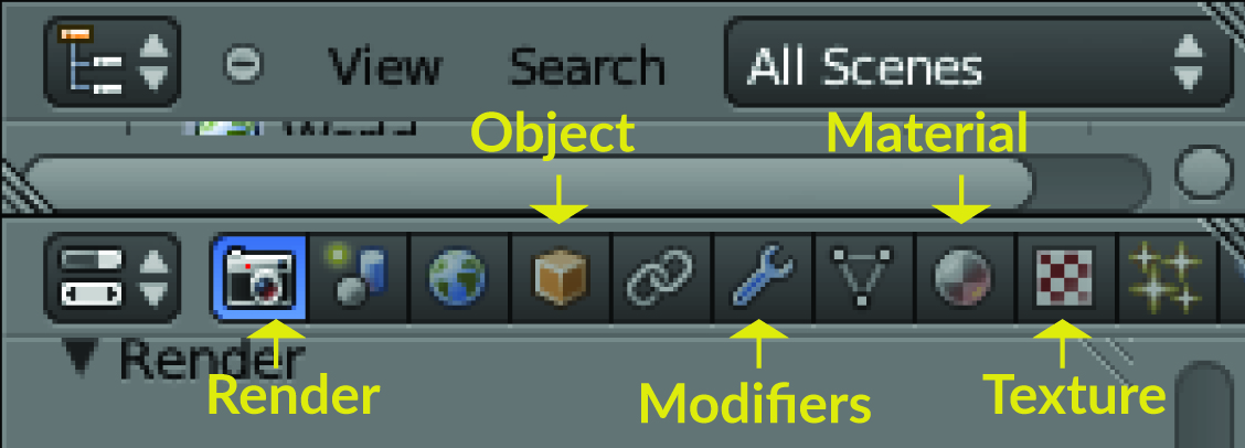 Properties panel Properties panel |
|---|
Note: Properties editor's interface is dynamically changing according to the selected object. For example, if you select the light, the little sun icon will appear to set the light properties and similarly you should select camera to be able to see the camera tab and modify the properties.
Object properties tab allows you to transform the location, orientation and scale of the object, along with their display properties. You can use numeric input for transformation parameters.
Example 3. Basic object transformation using properties modifier
- Make sure that Suzanne object is selected. It should be highlighted in outliner
- Go to Properties editor ‣ Object tab ‣ expand the Transform panel
- Type 3, 2, 4 for X, Y, Z parameters, respectively.
- Change Rotation and Scale parameters to see how they affect the object
Materials tab allows you to assign or change an object’s material. You can add and remove material, or use material browser to assign previously created materials to the object. In this tutorial we briefly introduce two basic components of Materials, Shaders and Textures.
Shading (or coloring) allows you to adjust the base color (as modified by the diffusion and specular reflection phenomenon) and the light intensity. You can also assign Texture to the objects, which is called Texture mapping. Texture mapping is often used to add detail to surfaces by projecting images and patterns onto those surfaces. Through the following examples we practice simple shading and texture mapping.
Example 4. Assigning simple Shaders and Textures
- Shaders
- From outlier select object make sure that Suzanne object is selected
- Go to properties editor ‣ object tab ‣ click on the + New button to create a new material
- Double click on the material name (e.g., Material.001) and change it to Mymat
- Expand the preview panel to see a live preview of the material as you are changing it
- Change the color parameter to red
- Go to 3D editor bottom Header ‣ Viewport shading ‣ rendered to see the object render in realtime
- Change the color to yellow
- Click on the Diffuse BSDF field in front of the surface parameter and select Glass BSDF
- Now try Emission BSDF and Glossy BSDF shaders while the viewport shader is on Rendered mode to see the effect on rendering. Your material preview and scene rendering should look like the figure shown below
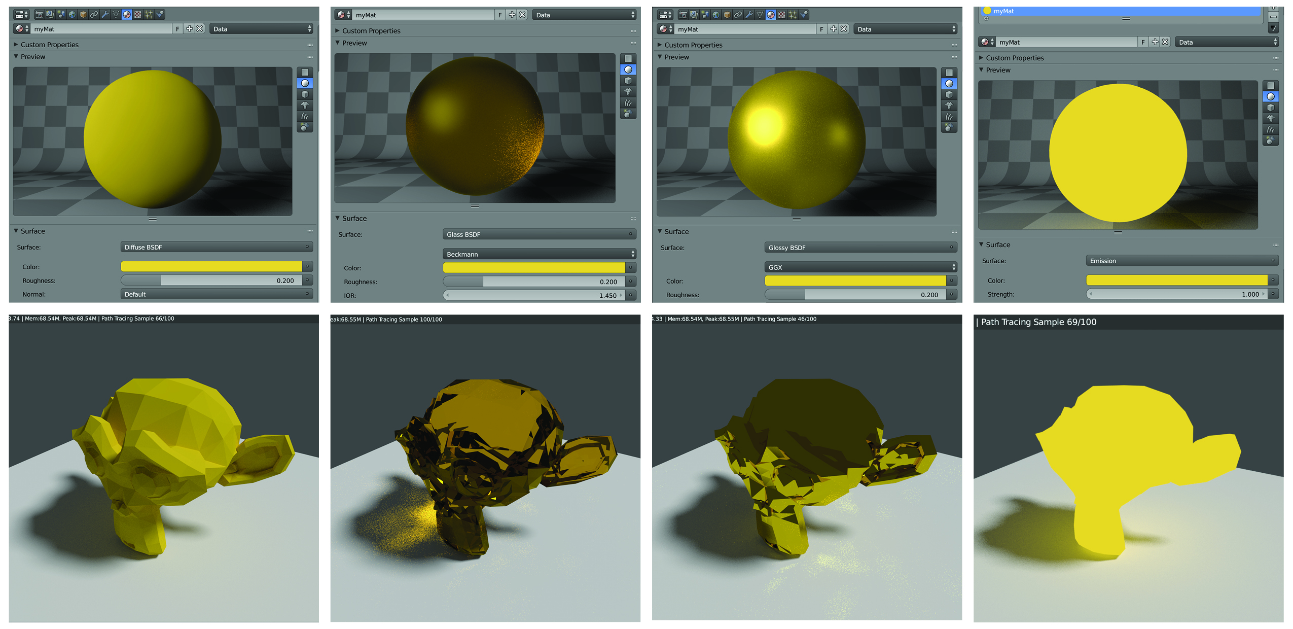 Left to right: Diffuse BSDF , Glass BSDF, Glossy BSDF, Emission
- Textures
- While the shader is still on “Glossy BSDF”, click on the radio button in front of the “Color” parameter. A widget with several columns will appear. From the texture column, select “Voronoi” to see how texture impact the rendering.
- Now try “Gradient” texture. Your material preview and scene rendering should look like the left two columns in the figure below.
 Left to right: Gradient texture, Voronoi texture, Glossy BSDF, Mix Shader
For creating more sophisticated materials you can use Node editor . Node editor is a visual interface for viewing and creating an interconnected network of nodes. In this network, each individual node performs some operation on the material, changing how it will appear when applied to the mesh, and passes it on to the next node. In this way, very complex material appearances can be achieved.
Example 5. Setup a Mix Shader using node editor.
In this example we mix a glossy shader with a diffuse shader to make a composite material.
- Right click on the Monkey object (Suzanne) to select it
- Switch the python console editor (bottom left area) to Node editor (figure below, left).
- In the node editor You will see the nodes we have already setup. The Glossy node shader’s output is connected to the surface input of the Material output.
We will now add two other shaders, a diffuse shader, and a mix shader. - From the Node Editor’s bottom Header ‣ Add ‣ Shader ‣ Diffuse BSDF
- From the Node Editor’s bottom Header ‣ Add ‣ Shader ‣ Mix shader. You should be able to see both nodes have been added in to your node editor.
- Change the color value of the Diffuse node to R: 0.075 G: 0.35 B: 0.50
- Disconnect the Glossy BSDF input from the surface
- Connect BSDF output of both Diffuse and Glossy shaders to the inputs on the left side of the Mix (Shader)
- Connect Shader output (on the right side) to the Surface input of the Material output nodes (figure below, right).
- With the Fac parameter, you can adjust the mixture level.
- Your material should look like the right column of the above figure learn more about nodes
 |
 Node design with mix shader Node design with mix shader |
|---|
Other Complementary resources for learning blender interface
In this section we will learn how to setup blender GIS addon and georeference the scene. We will also review the procedure for importing, processing and shading vector and raster data. We will proceed with the instructions using a simple viewshed assignment. Assignment goal is to visualize and compare viewshed simulations computed for 4 different locations across a site. The general workflow is as following.
I) Preparing the scene and lighting II) Georeferencing the scene III) Importing and processing the digital surface raster IV) Importing and processing the viewpoint shapefile V) Draping the viewshed map and orthophoto on the surface model
Note: Viewshed is a raster map showing a surface's visible areas from a given location.
There are two ways to complete the example; Scripting method (using blender's Python editor) and GUI (graphical user interface) method. For each step, the GUI procedure is listed as bullet points. Below that you can find the code snippet if you would like to follow the Scripting procedure. To execute the code snippet open a new text file in Text Editor and for each step directly copy-paste the code snippet into the editor and click on Run Script to execute the code.
| Method | Duration | difficulty |
|---|---|---|
| GUI | 1-2 hours | Complex |
| Python editor | 10-15 minutes | Easy |
Note For better learning complete the example with both methods but do not mix and match. Try to follow one method from the beginning to the end.
The first step is to clean the scene and setup rendering and lighting parameters.
GUI
- Run Blender and open the file Example_A.blend.
- Select the default Cube object in 3D viewport and delete it (right-click on the object ‣ press delete ‣ ok )
- Make sure that the render engine is set to "Cycles". You can find it in the top header, the default is Blender Render
- To increase the Lamp elevation and change the Lamp type to Sun for appropriate lighting:
- Left click on the Lamp object in Outliner to select it
- Go to Properties editor ‣ Object (the orange cube icon) ‣ Transform panel ‣ in the Location matrix, change the Z value to 1000 (see below figure if needed)
- For geospatial models you need a more powerful light source. To change lamp type to Sun and increase the emission:
- In Properties editor ‣ Lamp (two icons to the right of the Object icon) ‣ expand the Lamp panel ‣ Change lamp type to Sun
- Expand the Nodes panel ‣ Click on Use Nodes to enable modifying Sun parameters.
- Set the Strength parameter to 6.00
Python editor
import bpy
# remove the cube
cube = bpy.data.objects["Cube"]
cube.select = True
bpy.ops.object.delete()

# change lamp type and elevation
import bpy
lamp = bpy.data.lamps["Lamp"]
lamp.type = "SUN"
lampObj = bpy.data.objects["Lamp"]
lampObj.location[2] = 1000

# Setup node editor for lamp and increase the lamp power
lamp.use_nodes = True
lamp.node_tree.nodes["Emission"].inputs[1].default_value = 6

# Set render engine to cycles
bpy.context.scene.render.engine = 'CYCLES'
Changing the lamp elevation Changing the lamp elevation |
|---|
- Download the BlenderGIS addon
- Go to file ‣ user preferences (
Alt + Ctrl + U) ‣ Add-ons ‣ Install from File (bottom of the window) - Browse and select "BlenderGIS-master.zip" file
- You should be able to see the addon 3Dview: BlenderGIS added to the list. If not, type "gis" in the search bar while making sure that in the Categories panel All is selected. In the search results you should be able to see 3Dview: BlenderGIS. Select to load the addon.
- From the bottom of the preferences window click Save User Settings so the addon is saved and autmatically loaded each time you open blender
Before setting up the coordinate reference system of the Blender scene and configuring the scene projection, you should know the Coordinate Reference System (CRS) and the Spatial Reference Identifier (SRID) of your project. You can get the SRID from http://epsg.io/ or spatial reference website using your CRS. The example datasets in this exercise uses a NAD83(HARN)/North Carolina CRS (SSRID EPSG: 3358)
- In BlenderGIS add-on panel (in preferences windows), select to expand the 3D View: BlenderGIS
- In the preferences panel find Spatial Reference Systems and click on the + Add button
- In the add window put "3358" for definition and "NAD83(HARN)/North Carolina" for Description. Then select Save to addon preferences
- Select OK and close the User Preferences window
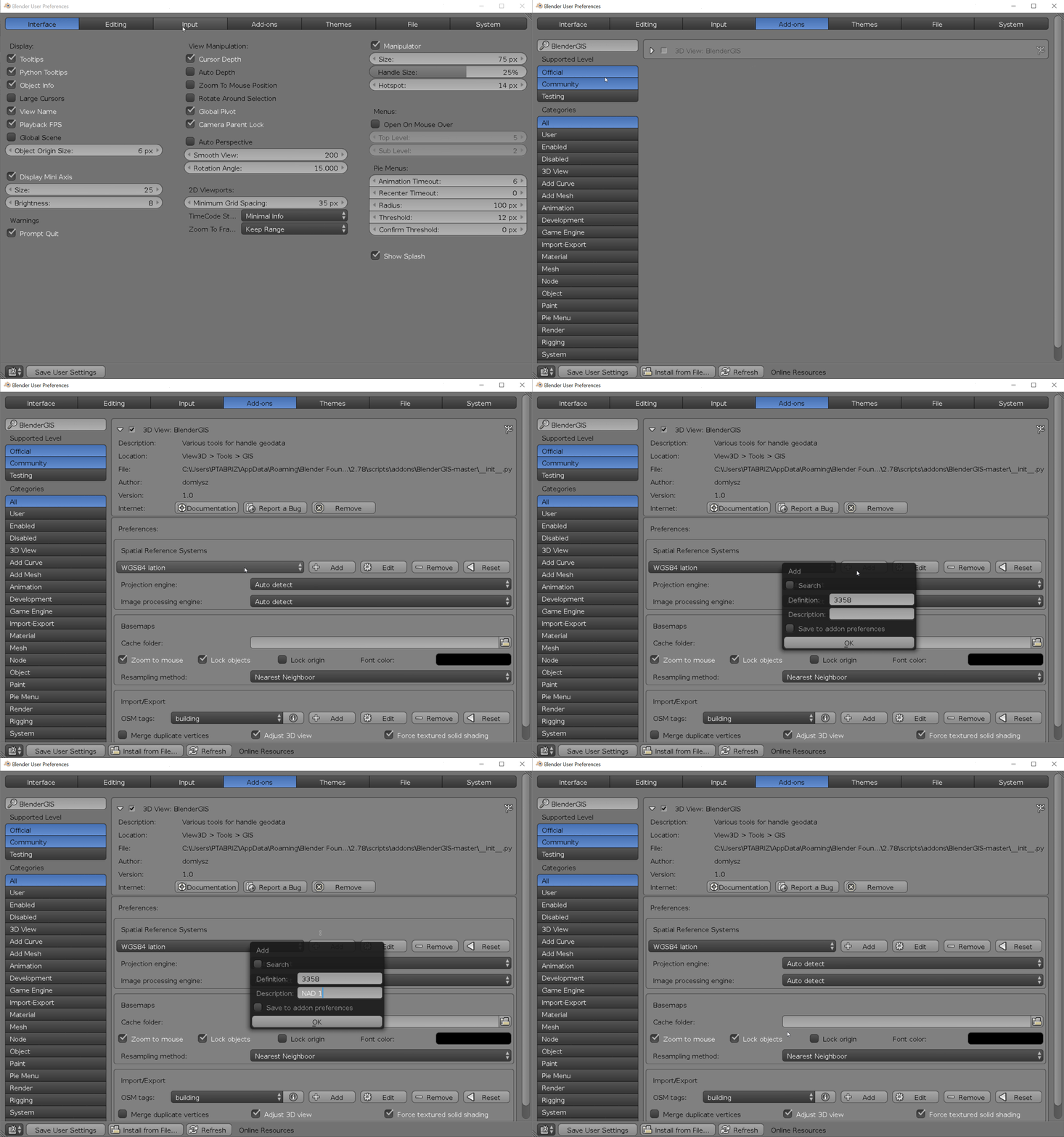 Installing addon and setting up Coordinate System Installing addon and setting up Coordinate System |
|---|
Learn more about Georefencing management in Blender
GUI
- Find and click on GIS addon’s interface in 3D viewport’s left toolbar. In the “Geoscene” panel , click on the gear shape icon and switch to NAD83(HARN), click ok.
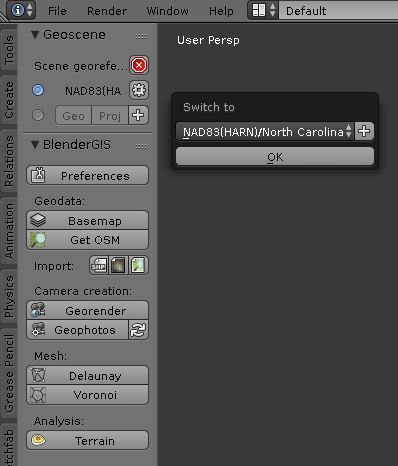 Georeferencing setup in Blender GIS |
|---|
Rasters can be imported and used in different ways. You can import them As DEM to use it as a 3D surface or as_Raw DEM_ to be triangulated or skinned inside Blender. You can select On Mesh to drape them as a texture on your 3D meshes. In this example, we import a digital surface model (DSM) derived from Lidar data points dataset as a 3D mesh using As DEM method. Note: Blender GIS imports both Digital Elevation Model (DEM) and Digital Surface Model (DSM) through As DEM method.
GUI
- Go to file ‣ import ‣ Georeferenced Raster
- On the bottom left side of the window find Mode and select As DEM
- Set subdivision to Subsurf and select NAD83(HARN) for georeferencing
- Browse to the 'workshop_material' folder and select 'example1_dsm.tif'
- Click on Import georaster on the top right header
- If all the steps are followed correctly, you should be able to see the terrain in 3D view window
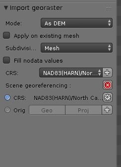 Georaster import parameters |
|---|
Python editor
import bpy
import os
filePath = os.path.dirname(bpy.path.abspath("//"))
fileName = os.path.join(filePath,'example1_dsm.tif')
bpy.ops.importgis.georaster(filepath=fileName,
                            importMode="DEM", subdivision="subsurf",
rastCRS="EPSG:3358")Usually when surface or elevation models are imported in Blender they are downsampled to a defaults subdivision resulting in smoothing out the surface details. The following procedure subdivides the imported mesh into smaller faces to enhance the surface representation. In this step we increase the subdivision units to acquire a more detailed surface.
GUI
- Select surface model (right click on the object)
- Go to 3D view editor's bottom toolbar ‣ Object interaction mode ‣ Edit Mode
- Switch to Face select
- If object is not orange in color (i.e., nothing is selected), go to Select ‣ (De)select All (or press
A) to select all faces (when the object faces are selected, they will turn orange) - Go to Tools (left toolbar) ‣ Mesh Tools ‣ Subdivide . The subdivide dialogue should appear on the bottom left on the toolbar. Type "4" in the number of cuts tab
- Go to 3D view editor's bottom toolbar ‣ Object interaction mode ‣ Object Mode . You should be able to see the surface details at this point (bottom figure, right image).
Python editor
import bpy
bpy.ops.object.mode_set(mode='EDIT')
bpy.ops.mesh.select_all(action='SELECT')
bpy.ops.mesh.subdivide(number_cuts=4, smoothness=0.2)
bpy.ops.object.mode_set(mode='OBJECT')
DSM surface after importing DSM surface after importing |
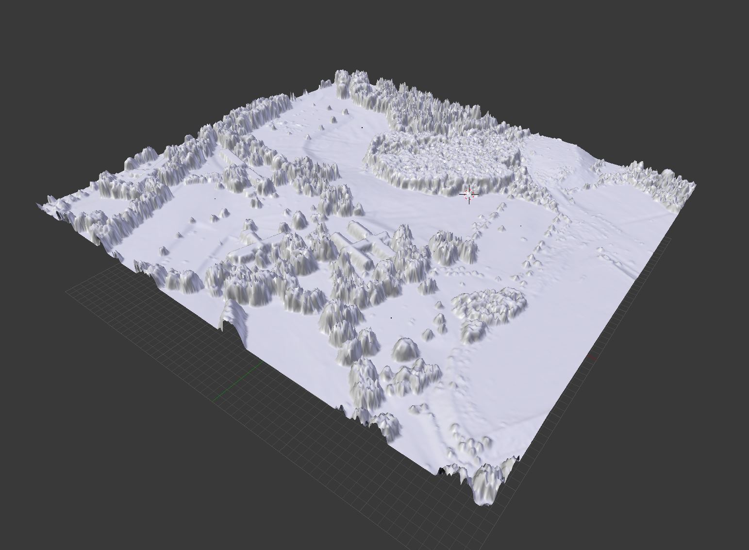 DSM surface after subdivision DSM surface after subdivision |
|---|
In this step we will import viewpoint locations as a point feature shapefile. With those features we can visualize the observer location from which the viewsheds are computed on the digital surface. BlenderGIS addon can import shape features respecting their attributes. In this example the "viewpoint.shp" has Elevation and Name attributes that we will use to assign hight and unique name to our viewshed points.
GUI
- To Import viewpoint shape file:
- Go to file ‣ import ‣ Shapefile
- Browse workshop data directory, select vpoints.shp and click on Import Shp . The shape import dialogue should appear in front of the GIS addon interface.
- Activate Elevation from field and in field panel select height
- Activate Separate objects
- Activate Object name from field and in field panel select Name, you should be able to see 4 the points on the surface and 4 objects added to the Outliner with the names Viewshed_1, Viewshed_2,Viewshed_3, Viewshed_4
- Select OK
 Blender Gis shape import dialogue |
|---|
Python editor
import bpy
import os
filePath = os.path.dirname(bpy.path.abspath("//"))
fileName = os.path.join(filePath,'vpoints.shp')
bpy.ops.importgis.shapefile(filepath=fileName, fieldElevName="height", fieldObjName='Name', separateObjects=True, shpCRS='EPSG:3358')Imported points are 2D vectors that cannot be rendered as they don't have actual surfaces. Now we create 4 small spheres and match their location with the imported points to visualize observer locations in 3D.
GUI
- To create spheres on the viewpoint location:
- Go to 3D Viewport’s bottom header ‣ Add ‣ Mesh ‣ UV sphere. The Add UV sphere dialogue will open on the left side of the Toolbar. Set the Size parameter to 3.000
- Select Sphere object (by clicking on it in Outliner) and press ctrl+c , ctrl+v to make a copy of the object, you should see the Sphere.001 in the outline. Make 3 copies of the sphere.
- In the outliner rename the sphere objects to Sphere1, Sphere2, ... , Sphere4. You can do that by clicking on the object name.
- From Outliner select the object Viewshed_1
- Go to Properties Editor ‣ Object ‣ Transform ‣ Location to retrieve the viewshed point’s coordinates (X,Y,Z)
- To move each of the 4 spheres to the corresponding viewshed location:
- Copy and paste the retrieved coordinates from Viewshed_1 into the location parameters for Sphere1
- Add 2.0 extra units to the Z parameter (only for Location) to raise the spheres above the ground
- Repeat this process for each Viewshed and each Sphere
- You should now have 4 spheres aligned on the imported viewshed points.
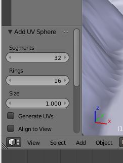 UV Sphere toolbar |
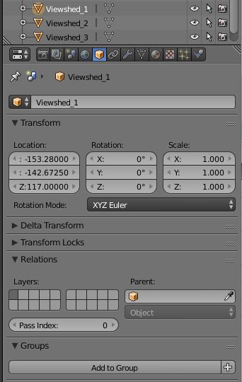 Object transform panel in properties editor |
|---|
Python editor
import bpy
# get viewpoint objects create a sphere using their X,Y and Z+2 coordinates
for obj in bpy.data.objects:
    if "Viewshed" in obj.name:
        bpy.ops.mesh.primitive_uv_sphere_add(size=3.0, location=(obj.location[0],obj.location[1],obj.location[2]+2))
        sphere = bpy.context.active_object
        # rename the sphere
        sphere.name = "Sphere" + obj.name[-2:]
4 spheres representing observation points |
|---|
In this step we create 3 additional copies of the surface model and move each of the viewpoint spheres to the
corresponding surface.
GUI
- Select DSM object and press
ctrl+c,ctrl+vto make a copy of the object , you should see the object example1_dsm.001 in the outliner - Select object example1_dsm001
- go to Properties Editor ‣ Object (cube icon)
- In the Transform panel ‣ Delta Transform ‣ X: type 750 to move the duplicated surface 750 meters to the east
- Create another copy of the DSM , put -750 for Y parameter to move the duplicate surface 750 meters to the south
- Create another copy of the DSM, put 750 for X parameter and -750 in Y parameter. The final model should look like figure
- Repeat the same procedure for the 4 Spheres (starting from Sphere 1) so each of them are moved to one of the surface.
Python editor
import bpy
for ob in bpy.data.objects:
ob.select = False
obj = bpy.data.objects["example1_dsm"]
obj.name = "example1_dsm1"
obj.select = True
# create and rename 3 replicates of DSM, and move spheres to create 4 DSMs and spheres
bpy.ops.object.duplicate_move(OBJECT_OT_duplicate={"mode":'TRANSLATION'}, TRANSFORM_OT_translate={"value":(750, 0, 0 )})
bpy.data.objects ["example1_dsm1.001"].name = "example1_dsm2"
sphere2Obj = bpy.data.objects ["Sphere_2"]
loc = sphere2Obj.location
sphere2Obj.location = (loc[0]+750, loc[1], loc[2])
bpy.ops.object.duplicate_move(OBJECT_OT_duplicate={"mode":'TRANSLATION'}, TRANSFORM_OT_translate={"value":(0, -750, 0 )})
bpy.data.objects ["example1_dsm2.001"].name = "example1_dsm3"
sphere3Obj = bpy.data.objects ["Sphere_3"]
loc = sphere3Obj.location
sphere3Obj.location = (loc[0]+750, loc[1]-750, loc[2])
bpy.ops.object.duplicate_move(OBJECT_OT_duplicate={"mode":'TRANSLATION'}, TRANSFORM_OT_translate={"value":(-750, 0, 0 )})
bpy.data.objects ["example1_dsm3.001"].name = "example1_dsm4"
sphere4Obj = bpy.data.objects ["Sphere_4"]
loc = sphere4Obj.location
sphere4Obj.location = (loc[0],loc[1]-750, loc[2])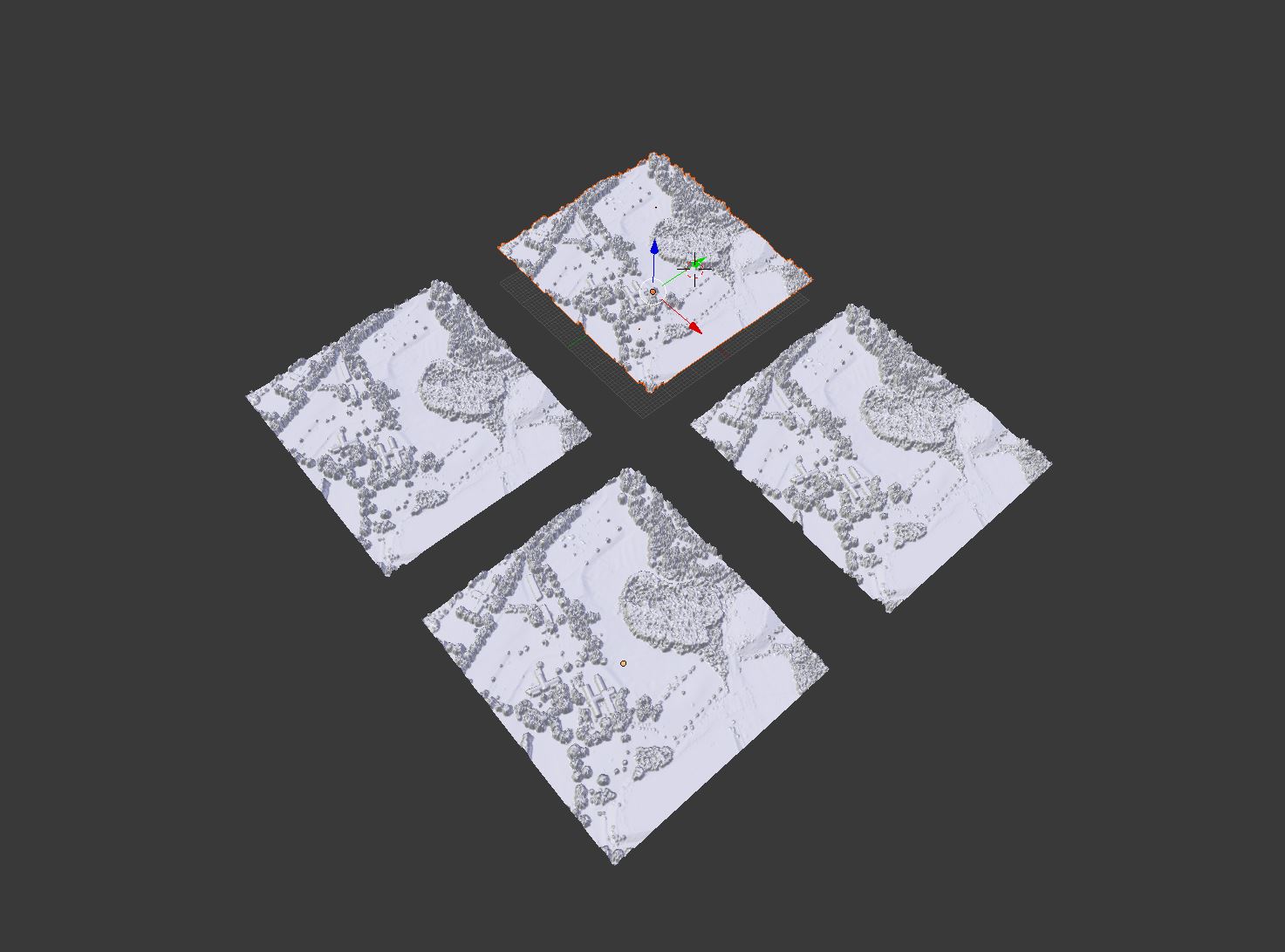 Replicated models Replicated models |
|---|
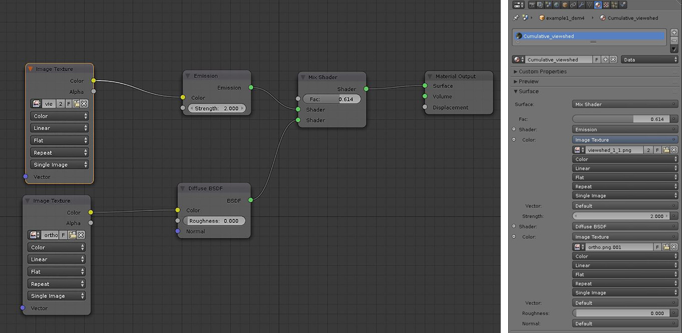
Now we will create a mixed material to combine Orthophoto and viewshed maps. We will use emission shaders to show viewsheds as glowing surfaces. For doing that we have created grayscale viewshed maps with black background, emmission shader assigns greater light emmission power to the lighter pixels.
GUI
- Make sure that the Render engine is set to Cycles and 3D viewport Shading is set to Material
- Change the bottom editor panel to Node editor. This can be done by simply changing the Editor Type selector (bottom left hand side of the window).
- Select the first DSM object "example_dsm1"
- Go to Properties tab ‣ Material Press + New button to add material
- Rename the Material to "Viewshed1"
- Expand the Surface panel and click on the gray square shaped icon on the right side of the Surface parameter to see a popup window with texture parameters. Select Mix Shader . You should be able to see two Shaders added below the mix shader.
- Click on the first shader and select Emission from the dropdown list
- Click on the radio button on the right side of the color field ‣ texture ‣ Image texture
- Click on Open and load "viewshed_1_1.png". You should be able to see the viewshed draped on the DSM surface
- Change the Strength slider to 1.8 to increase the viewshed's emission power
- Click on the second shader and select Diffuse BSDF from the dropdown list
- Click on the radio button on the right side of the color field ‣ texture ‣ Image texture
- Click on Open and load "ortho.png". You should be able to see the viewshed draped on the DSM surface
Now notice how the material logic and workflow is represented in Node editor. You can play with each of the individual nodes ,the links between them and the values.
- Play with the Fac slider on the Mix shader node to adjust the mixture level
- To repeat the shading procedure for the other 3 objects using "Viewshed_2_1.png", "Viewshed_3_1.png", "Viewshed_4_1.png"
- Select the Surface object and Go to Properties tab ‣ Material Press on whirpool shaped button (next to new botton) to browse and load "Viewshed 1" matarial. Make a new copy of the material by pressing the number button on the left side of the material name field. Rename the new material to "Viewshed 2".
- Now either from the Node editor or in the Material tab change the emmission texture to "viewshed_2_1.png"
- Repeat the same procedure for two other surfaces.
 Node editor and Properties panel Node editor and Properties panel |
|---|
Python editor
import bpy
import os
filePath = os.path.dirname(bpy.path.abspath("//"))
ortho = os.path.join(filePath, 'ortho.png')
for obj in bpy.data.objects:
if "dsm" in obj.name :
obj.select = True
fileName = "viewshed_{0}_1.png".format(obj.name[-1:])
matName = os.path.join(filePath, fileName)
# Create a new material and assign it to the DSM object # 3
mat = (bpy.data.materials.get(matName) or
bpy.data.materials.new(matName))
obj.data.materials.append(mat)
# Get material tree , nodes and links #
mat.use_nodes = True
node_tree = mat.node_tree
nodes = node_tree.nodes
links = node_tree.links
for node in nodes:
nodes.remove(node)
diffuseNode = node_tree.nodes.new("ShaderNodeBsdfDiffuse")
diffuseNode.location = (300,400)
#diffuseNode = nodes["Diffuse BSDF"]
# Add a new texture for viewshed #
viewshedNode = node_tree.nodes.new("ShaderNodeTexImage")
viewshedNode.select = True
node_tree.nodes.active = viewshedNode
viewshedNode.image = bpy.data.images.load(matName)
viewshedNode.location = (100, 100)
# Add a new texture for ortho #
orthoNode = node_tree.nodes.new("ShaderNodeTexImage")
orthoNode.select = True
node_tree.nodes.active = orthoNode
orthoNode.image = bpy.data.images.load(ortho)
orthoNode.location = (100, 400)
# Add a new mixshader node and link it to the diffuse color node#
mixShaderNode = node_tree.nodes.new("ShaderNodeMixShader")
mixShaderNode.location = (600, 250)
mixShaderNode.inputs["Fac"].default_value = .7
emissionNode = node_tree.nodes.new("ShaderNodeEmission")
emissionNode.location = (300, 100)
outputNode = node_tree.nodes.new("ShaderNodeOutputMaterial")
outputNode.location = (800, 250)
emissionNode.inputs[1].default_value = 2
links.new (viewshedNode.outputs["Color"], emissionNode.inputs["Color"])
links.new (orthoNode.outputs["Color"], diffuseNode.inputs["Color"])
links.new (emissionNode.outputs["Emission"], mixShaderNode.inputs[2])
links.new (diffuseNode.outputs["BSDF"], mixShaderNode.inputs[1])
links.new (mixShaderNode.outputs["Shader"], outputNode.inputs["Surface"])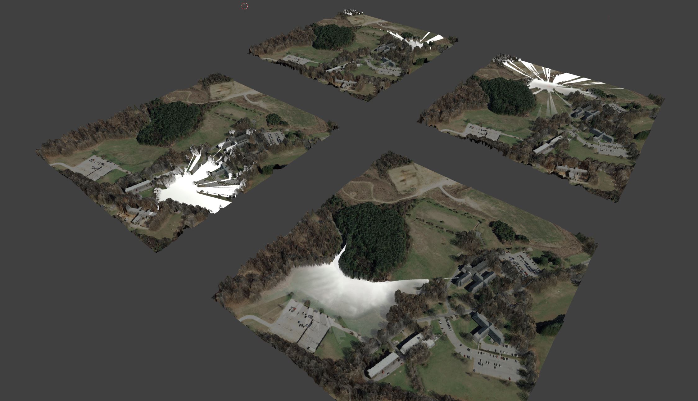 Viewshed and Orthophoto draped on DSM surface using Mix shader Viewshed and Orthophoto draped on DSM surface using Mix shader |
|---|
Now follow the same workflow to shade viewpoint spheres but this time only use diffuse node (Diffuse BSDF) a with solid orange color.
‣ GUI
- Select the first sphere, create a new material using Diffuse BSDF
- Change the surface color to orange
- Load the material in all sphere objects
import bpy
for obj in bpy.data.objects:
if "Sphere" in obj.name:
obj.select = True
matName = "sphere"
# Create a new material and assign it to the DSM object # 3
mat = (bpy.data.materials.get(matName) or
bpy.data.materials.new(matName))
obj.data.materials.append(mat)
# Get material tree , nodes and links #
mat.use_nodes = True
node_tree = mat.node_tree
nodes = node_tree.nodes
links = node_tree.links
nodes[1].inputs[0].default_value = (.8, .3, 0, 1)
obj.select = False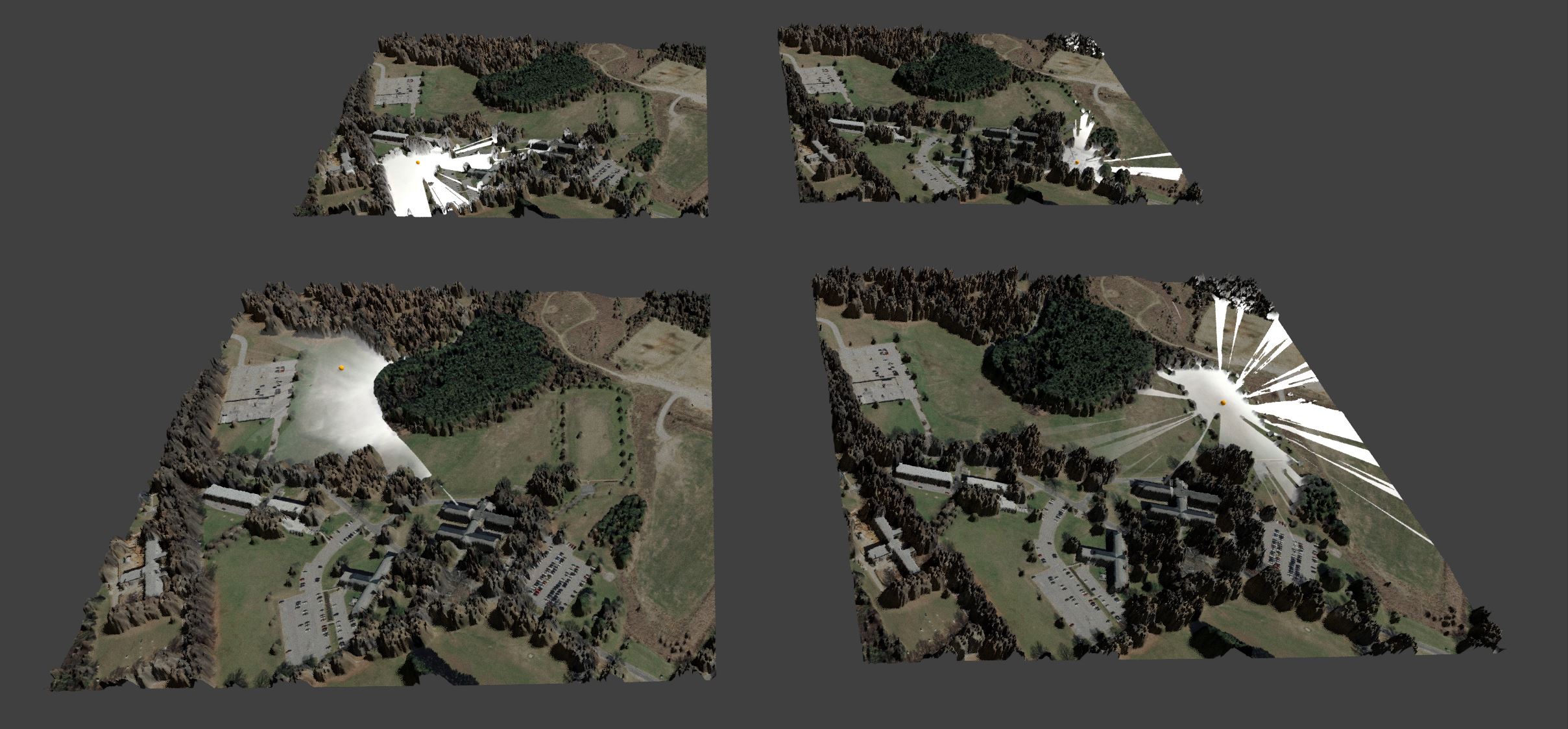 Viewport render of the viewshed |
|---|
Now lets try to run the entire procedure with a python file using Text editor and Python console
‣ GUI
- From top header goto file‣ New to Open a fresh copy of Blender
- Save the blender file with you preferred name in the workshop directory. Note: This is an important step since your all the paths in python code are linked to that directory
- In the top header find Layout (right next to help ) and switch the layout to Scripting The scripting layout includes : a Text editor(left), a Python Console (bottom) and 3D view (right)
- Procedure for Text editor
- In Text editor ‣ Open ‣ Go to workshop directory and find example_a.py
- Click on run script
- Procedure for Python Console
- type the following lines in the console. Note that you need to type in the workshop path in you computer in the first line.
Python Console>>>
filename = "/full/path/to/example_a.py"
exec(compile(open(filename).read(), filename, 'exec'))
Python editor
import bpy
import os

filePath = os.path.dirname(bpy.path.abspath("//"))
dsmName = os.path.join(filePath,'example1_dsm.tif')
imgPath = os.path.join(filePath,'cumulative_viewshed.png')
vpointName = os.path.join(filePath,'vpoints.shp')
ortho = os.path.join(filePath, 'ortho.png')

# Setting up the scene
if bpy.data.objects.get("Cube"):
    cube = bpy.data.objects["Cube"]
    cube.select = True
    bpy.ops.object.delete()

# change lamp type and elevation
import bpy
lamp = bpy.data.lamps["Lamp"]
lamp.type = "SUN"
lampObj = bpy.data.objects["Lamp"]
lampObj.location[2] = 1000

# Setup node editor for lamp and increase the lamp power
lamp.use_nodes = True
lamp.node_tree.nodes["Emission"].inputs[1].default_value = 6

# Set render engine to cycles
bpy.context.scene.render.engine = 'CYCLES'
bpy.ops.importgis.georaster(filepath=dsmName,
                            importMode="DEM", subdivision="subsurf",
                            rastCRS="EPSG:3358")

# Subdivision render engine to cycles
bpy.ops.object.mode_set(mode='EDIT')
bpy.ops.mesh.select_all(action='SELECT')
bpy.ops.mesh.subdivide(number_cuts=4, smoothness=0.2)
bpy.ops.object.mode_set(mode='OBJECT')

# import viewpoints
bpy.ops.importgis.shapefile(filepath=vpointName,fieldElevName="height",fieldObjName='Name',separateObjects=True,shpCRS='EPSG:3358')

# adding spheres
for obj in bpy.data.objects:
    if "Viewshed" in obj.name:
        bpy.ops.mesh.primitive_uv_sphere_add(size=3.0, location=(obj.location[0],obj.location[1],obj.location[2]+2))
        sphere = bpy.context.active_object
        # rename the sphere
        sphere.name = "Sphere" + obj.name[-2:]

for ob in bpy.data.objects:
    ob.select = False
obj = bpy.data.objects["example1_dsm"]
obj.name = "example1_dsm1"
obj.select = True

# create and rename 3 replicates of DSM, and move spheres to create 4 DSMs and spheres

bpy.ops.object.duplicate_move(OBJECT_OT_duplicate={"mode":'TRANSLATION'}, TRANSFORM_OT_translate={"value":(750, 0, 0 )})
bpy.data.objects ["example1_dsm1.001"].name = "example1_dsm2"
sphere2Obj = bpy.data.objects ["Sphere_2"]
loc = sphere2Obj.location
sphere2Obj.location = (loc[0]+750, loc[1], loc[2])

bpy.ops.object.duplicate_move(OBJECT_OT_duplicate={"mode":'TRANSLATION'}, TRANSFORM_OT_translate={"value":(0, -750, 0 )})
bpy.data.objects ["example1_dsm2.001"].name = "example1_dsm3"
sphere3Obj = bpy.data.objects ["Sphere_3"]
loc = sphere3Obj.location
sphere3Obj.location = (loc[0]+750, loc[1]-750, loc[2])

bpy.ops.object.duplicate_move(OBJECT_OT_duplicate={"mode":'TRANSLATION'}, TRANSFORM_OT_translate={"value":(-750, 0, 0 )})
bpy.data.objects ["example1_dsm3.001"].name  = "example1_dsm4"
sphere4Obj = bpy.data.objects ["Sphere_4"]
loc = sphere4Obj.location
sphere4Obj.location = (loc[0],loc[1]-750, loc[2])

# Shading Viewsheds
for obj in bpy.data.objects:
    if "dsm" in obj.name :
        obj.select = True
        fileName = "viewshed_{0}_1.png".format(obj.name[-1:])
        matName = os.path.join(filePath, fileName)
# Create a new material and assign it to the DSM object # 3

        mat = (bpy.data.materials.get(matName) or
               bpy.data.materials.new(matName))

        obj.data.materials.append(mat)

        # Get material tree , nodes and links #
        mat.use_nodes = True
        node_tree = mat.node_tree
        nodes = node_tree.nodes
        links = node_tree.links
        for node in nodes:
            nodes.remove(node)
        diffuseNode = node_tree.nodes.new("ShaderNodeBsdfDiffuse")
        diffuseNode.location = (300,400)
        #diffuseNode = nodes["Diffuse BSDF"]

        # Add a new texture for viewshed #
        viewshedNode = node_tree.nodes.new("ShaderNodeTexImage")
        viewshedNode.select = True
        node_tree.nodes.active = viewshedNode
        viewshedNode.image = bpy.data.images.load(matName)
        viewshedNode.location = (100, 100)

        # Add a new texture for ortho #
        orthoNode = node_tree.nodes.new("ShaderNodeTexImage")
        orthoNode.select = True
        node_tree.nodes.active = orthoNode
        orthoNode.image = bpy.data.images.load(ortho)
        orthoNode.location = (100, 400)
        # Add a new mixshader node and link it to the diffuse color node#

        mixShaderNode = node_tree.nodes.new("ShaderNodeMixShader")
        mixShaderNode.location = (600, 250)
        mixShaderNode.inputs["Fac"].default_value = .7
        emissionNode = node_tree.nodes.new("ShaderNodeEmission")
        emissionNode.location = (300, 100)
        outputNode = node_tree.nodes.new("ShaderNodeOutputMaterial")
        outputNode.location = (800, 250)
        emissionNode.inputs[1].default_value = 2

        links.new (viewshedNode.outputs["Color"], emissionNode.inputs["Color"])
        links.new (orthoNode.outputs["Color"], diffuseNode.inputs["Color"])
        links.new (emissionNode.outputs["Emission"], mixShaderNode.inputs[2])
        links.new (diffuseNode.outputs["BSDF"], mixShaderNode.inputs[1])
        links.new (mixShaderNode.outputs["Shader"], outputNode.inputs["Surface"])
# shading viewpoints
for obj in bpy.data.objects:
    if "Sphere" in obj.name:
        obj.select = True
        matName = "sphere"
    # Create a new material and assign it to the DSM object # 3
        mat = (bpy.data.materials.get(matName) or
               bpy.data.materials.new(matName))
        obj.data.materials.append(mat)
        # Get material tree , nodes and links #
        mat.use_nodes = True
        node_tree = mat.node_tree
        nodes = node_tree.nodes
        links = node_tree.links
        nodes[1].inputs[0].default_value = (.8, .3, 0, 1)
        obj.select = False

# Switch to shading mode
for area in bpy.context.screen.areas:
    if area.type == 'VIEW_3D':
          for space in area.spaces:
              if space.type == 'VIEW_3D':
space.viewport_shade = 'MATERIAL'In this section we learn the basics to setup simple coupling for importing and processing of geospatial data, in realtime. We do that by setting up a monitoring system inside blender that continuously looks for incoming commands (e.g, through sockets), files (e.g, shape file, raster files, etc.), or user interaction (e.g, mouse, joystick, keyboard). In Blender this procedure is handled through a module called Modal Timer Operator. The reason that we focus on this specific module is that routine monitoring libraries like Watchmode or Threading are not well handled in Blender and often results in crashes. These modules interfere with blender's ability to run multiple operators at once and update different parts of the interface as the tool runs.
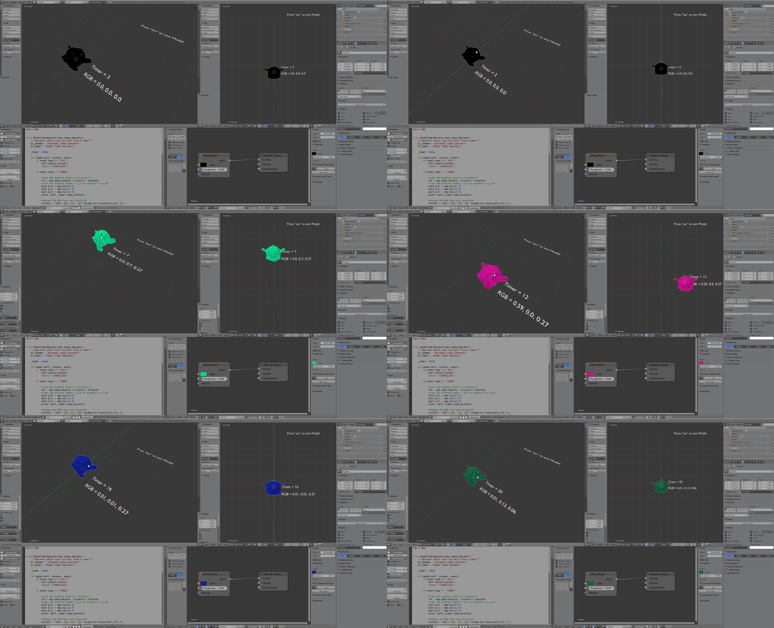
The data can be transferred locally or over network, using simple file copy or more advanced methods like sockets. As an example, the following video shows a real-time coupling with GRASS GIS. GrassGIS itself is paired with Kinect to scan the elevation and color changes in the physical model. As user interacts with the physical model, GRASS GIS runs various simulations, and exports them as raster and shape formats to a system directory. In Blender Modal timer is continuously monitoring the directory to update the model based on incoming data types. Those include terrain surface (Geotiff), ponding simulation (3Dpolygon), landcover patches (3D polygon), camera location (3Dpolyline), trail (3Dpolyline).
 Modal timer example Modal timer example |
|---|
Example 1.
Lets take a peek at the module's components and functionality in the following example.
‣ Procedure
-
Open the file Modal.blend
-
Run the script that is loaded in the text editor
-
Select the Monkey object and move it around. You will see that as you are moving the object, three operations are running simultaneously: 1) the RGB values change, 2) a text object changes to show the updated RGB values, 3) and the timer text object changes to show the elapsed time in seconds.
-
Cancel the modal mode using "Esc" key.
-
Take a quick look at the commented code to check the modules components and their functionality
import bpy

class ModalTimerOperator(bpy.types.Operator):
    """Operator which runs its self from a timer"""
    bl_idname = "wm.modal_timer_operator"
    bl_label = "Modal Timer Operator"

    _timer = None

    def modal(self, context, event):

        # Terminate module when ESC key is pressed
        if event.type in {'ESC'}:
            self.cancel(context)
            return {'CANCELLED'}

        # assign timer condition to event handler
        if event.type == 'TIMER':

            # get the suzanne object's location #
            loc = bpy.data.objects ["Suzanne"].location
            # set the diffuse shader r,g,b to suzanne's x,y,z#
            self.a[0] = abs(loc[0]/5)
            self.a[1] = abs(loc[1]/5)
            self.a[2] = abs(loc[2]/5)
            print (self._timer.time_duration)

            #update the RGB text and location#
            colText = "RGB = {0}, {1}, {2}".format(str(round(self.a[0],2)),
                            str(round(self.a[1],2)),str(round(self.a[2],2)))
            self.rgb.data.body = colText
            self.rgb.location = (loc[0]+1,loc[1]-.5,loc[2]-1)

            #update the timer text and location#
            self.timer_text.location = (loc[0]+1,loc[1]+.5,loc[2]-1)
            self.timer_text.data.body = "Timer = " + str(round(self._timer.time_duration))

        return {'PASS_THROUGH'}

    def execute(self, context):
        wm = context.window_manager
        # Per seconds timer steps
        self._timer = wm.event_timer_add(1, context.window)
        wm.modal_handler_add(self)

        self.timer_text = bpy.data.objects ["Timer"]
        self.rgb = bpy.data.objects ["RGB"]
        # get the active object material #
        mat = bpy.data.materials.get("Material")
        # Get diffuse shader nodes's color #
        node_tree = mat.node_tree
        self.a = node_tree.nodes["Diffuse BSDF"].inputs[0].default_value

        return {'RUNNING_MODAL'}

    def cancel(self, context):
        wm = context.window_manager
        wm.event_timer_remove(self._timer)


def register():
    bpy.utils.register_class(ModalTimerOperator)


def unregister():
    bpy.utils.unregister_class(ModalTimerOperator)


if __name__ == "__main__":
    register()

    # test call
bpy.ops.wm.modal_timer_operator()In this example we are using modal timer to monitor a system directory, In the workshop_materials folder you can see two folders named "Watch" and "scratch". The scratch folder contains 45 shape files and 45 images. The shapefiles represent viewpoints across a path, and textures represent viewsheds simulated from those locations. Viewsheds are combined with landcover to show the landuse composition of visible surface. Through a python script we setup modal timer to constantly look for files to import and process. To emulate the geospatial simulation we setup a second modal timer that copies the geospatial data from the Scratch folder to Watch folder (look at above scheme). The python script is consisted of the following python classes.
- Locate and run coupling_example.blend in workshop_materials
1. adapt class processes the incoming files and scene objects. Specifically it performs the following operations.
- Imports the viewshed map
- Replaces the emission texture of the DSM object with the imported map
- Imports the viewpoint shape file
- Aligns the location of the viewshed marker (Torus object) with the location of the imported viewpoint.
2. Modal timer Looks into the Watch directory, detects the type of incoming file, sends them to adapt class and finally removes the file from the watch folder.
3. Modal_copy acts as a surrogate for your GIS software and copies texture and Point shape files from Scratch folder to the Watch folder to simulate the condition where your GIS application is automatically sending files over the network or locally.
4. Panel a small widget with buttons to run the modules (2 and 3)
‣ Procedure
- Go to file ‣ preferences ‣ addons ‣ BlenderGIS ‣ import/Export panel
- Unselect Adjust 3D view and Forced Textured solid shading.
- Now run the script loaded into the text editor
- The scripts adds a new panel in 3D view's toolbar (left side) with two buttons, Watch mode and Copy files
- First Press Watch mode and then press Copy files
- You should be able to see the viewshed maps and the observer location object updating along the path.
class adapt:
    ''' Adapt the scene objects based on viewpoint and texture files'''

    def __init__(self):
        self.terrain = "DSM"
        self.viewpoint = "Torus"
        filePath = os.path.dirname(bpy.path.abspath("//"))
        fileName = os.path.join(filePath,'vpoints.shp')

    def viewshed(self,texture,vpoint):
        ''' Recieve and process viewshed point shape file and texture '''

        ## import the shapefile, move viewmarker and delete the shapefile ##
        vpointDir = os.path.join (watchFolder,vpoint)
        vpointFile = vpointDir + "/" + vpoint + ".shp"
        if not bpy.data.objects.get(vpoint):
            bpy.ops.importgis.shapefile(filepath=vpointFile,fieldElevName="elev",
            shpCRS='EPSG:3358')

        bpy.data.objects[self.viewpoint].location = bpy.data.objects[vpoint].location
        shutil.rmtree(vpointDir)

        ## assign change terrain's texture file ##
        if bpy.data.objects.get(self.terrain):
            bpy.data.objects[self.terrain].select = True
            # remove the texture file from the directory
            os.remove(os.path.join(watchFolder,texture))

        # Change the material emmission shader texture #
        if not bpy.data.images.get(texture):
            texpath = os.path.join(scratchFolder,texture)
            bpy.data.images.load(texpath)
        # get the active object material #
        mat = bpy.data.materials.get("Material")
        # Get material tree , nodes and links #
        nodes = mat.node_tree.nodes
        nodes.active = nodes[5]
        #Replace the texture #
        nodes[5].image = bpy.data.images[texture]
class Modal_watch(bpy.types.Operator):
"""Operator which interatively runs from a timer"""
bl_idname = "wm.loose_coupling_timer"
bl_label = "loose coupling timer"
_timer = 0
_timer_count = 0
def modal(self, context, event):
if event.type in {"RIGHTMOUSE", "ESC"}:
return {"CANCELLED"}
# this condition encomasses all the actions required for watching
# the folder and related file/object operations
if event.type == "TIMER":
if self._timer.time_duration != self._timer_count:
self._timer_count = self._timer.time_duration
fileList = (os.listdir(watchFolder))
# Tree patches #
for fileName in fileList:
if ".png" in fileName:
vpoint = "viewpoint_" + fileName.split(".")[0]
if vpoint in fileList:
adapt().viewshed(fileName,vpoint)
self.adaptMode = "VIEWSHED"
return {"PASS_THROUGH"}
def execute(self, context):
bpy.context.space_data.show_manipulator = False
wm = context.window_manager
wm.modal_handler_add(self)
self._timer = wm.event_timer_add(3, context.window)
self.adaptMode = None
return {"RUNNING_MODAL"}
def cancel(self, context):
wm = context.window_manager
wm.event_timer_remove(self._timer)class Modal_copy(bpy.types.Operator):
"""Operator which interatively runs from a timer"""
bl_idname = "wm.copy_files"
bl_label = "copy files to watch folder"
_timer = 0
_timer_count = 0
_index = 0
def modal(self, context, event):
if event.type in {"RIGHTMOUSE", "ESC"}:
return {"CANCELLED"}
if event.type == "TIMER":
if self._index == len(self.copyList):
self._index = 0
if self._timer.time_duration != self._timer_count:
if self.copyList and not os.listdir(watchFolder):
item = self.copyList[self._index]
if item not in self._copiedList:
fileSrc = os.path.join(scratchFolder, item[1])
fileDst = os.path.join(watchFolder, item[1])
dirSrc = os.path.join(scratchFolder, item[2])
dirDst = os.path.join(watchFolder, item[2])
shutil.copytree(dirSrc, dirDst)
shutil.copyfile(fileSrc, fileDst)
self._copiedList.append(item)
self._index += 1
return {"PASS_THROUGH"}
def execute(self, context):
wm = context.window_manager
wm.modal_handler_add(self)
self._timer = wm.event_timer_add(1, context.window)
fileList = os.listdir(scratchFolder)
self._copiedList = []
self.copyList = []
for f in fileList:
if ".png" in f:
vpointDir = "viewpoint_" + f.split(".")[0]
if vpointDir in fileList:
self.copyList.append((int(f.split(".")[0]),f,vpointDir))
self.copyList = sorted(self.copyList)
return {"RUNNING_MODAL"}
def cancel(self, context):
wm = context.window_manager
wm.event_timer_remove(self._timer)Blend4Web is a powerful tool for easy publishing and sharing your data online, inside blender. Specially for non-coders, the addon is a convenient tool to create sophisticated interactive models. To take a peek of the Blend4Web functionalities, look at the following applications featured in Blend4Web examples library.
Everest
Low poly rendering
Example . Isosurfaces
In this example we use Blend4Web addon to export a 3D model online. The sample data is borrowed from a project focused on visualizing spatio-temporal patterns of pedestrian behavior using data gathered from public webcams. The data is visualized using an Isosurface created in Paraview. The shape of an isosurface shows the spatio-temporal evolution of pedestrian density. The time axis is represented as a color ramp draped over the isosurface.
‣ Procedure
- From the workshop_materials directory locate and open isosurface.blend
- To setup Blend4Web addon
- Go to File ‣ Preferences ‣ addons ‣ install from file
- From the workshop_materials directory locate and select blend4web_addon_17_06.zip
- Make sure that the addon is setup and selected
- Click save user settings and close the preferences window
‣ Procedure
-
To export the blender scene as .html using GUI
- Go to File ‣ Export ‣ Blend4Web(.html)
- Name your file and click on B4W Export HTML button
- Double click on the html file to open it in the browser
-
To export the blender scene as .html using editor
- run the script in the text editor
Blend4Web interface - run the script in the text editor
This work is built upon great contributions and support of Blender team, Blender GIS addon developers (domlysz/BlenderGIS) , Center for Geospatial Analytics, NC State's Geoforall lab and Garrett Millar.


