CIFAR10 classification experiments

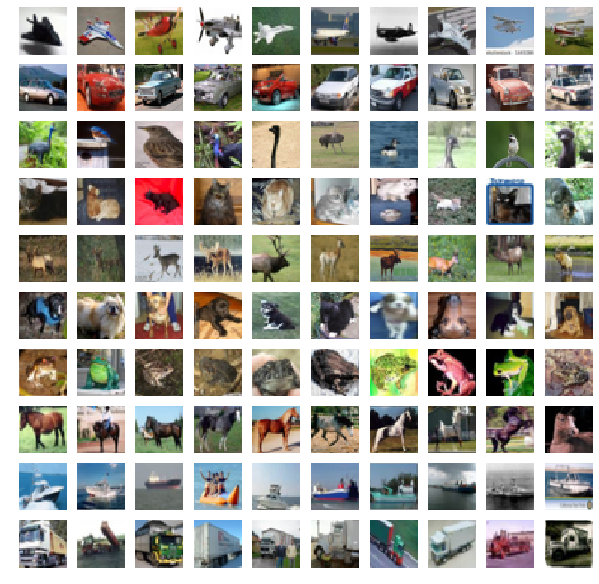
Here we present our experiments with classification of images from CIFAR-10 dataset.

Dataset

CIFAR-10 database consists of 60000 color images in 10 classes ['plane','auto','bird','cat','deer','dog','frog','horse','ship','truck']. Each image is of the size 32x32 with RGB features, so the single data sample has 32x32x3=3072 features.

The dataset is partitioned to training (50000) and testing (10000) samples.

Loading dataset

The script myutils.py provides very simple procedure for (down)loading the data.

import myutils
data_training, data_testing = myutils.load_CIFAR_dataset()

When loaded, data_training is a list of training images and its labels. For example, the $k$-th image is stored in the array data_training[k][0] (with shape (32,32,3)) and its label is data_training[k][1] (integer number in range(10)).

Some example images

The iPython notebook CIFAR10-visualization.ipynb presents some examples images from each of 10 classes in CIFAR10.

Classification

In our case, the classification problem means the supervised learning using only the training data (50000 images of CIFAR10). We measure the accuracy of any model using testing data.

Of course there are many approaches to the classification problem. Here we applied the feature extraction preprocessing approach in order to finally build the linear classifiers to learn the new (possibly separable) features. One can try to use nonlinear techniques, as well. However our goal is to build (possibly using nonlinear techniques) such features to be finally simply separable by linear classifier.

HOG features

The first approach extracts features using histograms of oriented gradients of the images.

This approach does not give spectacular results. We obtained the accuracy about 49--51% on top of HOG features; see Classification_using_HOG_features.ipynb for more details. This is far from the best results in CIFAR10 classification challenge; see Rodrigo Benenson's ranking

Transfer learning

The top results in considered classification problem are obtained using the convolutional neural networks (CNN in short). However, the process of training such (deep?) network is very time consuming; usually requires at leat one GPU unit and takes hours/days/weeks. One can find a lot of CNN models in Internet and try to train them on CIFAR10 dataset.

In this project we use the approach named transfer learning, which means that we take already pretrained CNN (possibly deep) on some database of images. This database does not necessarily need to be CIFAR10, Moreover, such CNN can be trained to classify images from much more classes than 10. More precisely the transfer learning can be performed in two way:

1. Extract features using CNN - perform the prediction of CIFAR10 with CNN but without the last layer (usually softmax) in order to obtain somehow complex features (called CNN codes).
2. Fine-tuning the CNN parameters - perform the process of further learning of CNN but with CIFAR10 images. One should modify the last layer (usually softmax) of the network, which is responsible for the classification (probably with much more classes). The examples CNN models trained on huge database --- ImageNET (14*10^6 images, 1000 classes) can be found in tensorflow project github repo

Here we used the first approach. More precisely, we extracted the CNN codes of CIFAR10 training and testing images using the following networks (all pretrained on ImageNET):

• ResNET50
• VGG16
• VGG19
• Inception v3

Feature extraction using keras

The notebook Feature_extraction_using_keras.ipynb provides the python code for the extraction process. All the CNN models (pretrained as well) are available via keras library. In our case the extraction used TensorFlow backend.

Our hardware setup is GPU (nVIDIA GTX 1050 Ti 4GB). Everything worked in Ubuntu 17.04. All the models above give the accuracy range 70--91% on testing dataset. The best result (91.58%) was achieved by classification of the features extracted using ResNET50 network.

We used both PCA and tSNE decompositions into 2 dimensions in order to visualize the features. The figure below presents the tSNE visualization of features extracted by fine-tuned ResNET50 network

Feature extraction using Inception_v3 from TensorFlow

We also used the TensorFlow checkpoint of Inception v3 network available with the URL http://download.tensorflow.org/models/image/imagenet/inception-2015-12-05.tgz

The archive contains the file classify_image_graph_def.pb with Inception_v3 network (also pretrained on ImageNET), which has different weights than Inception_v3 model from keras.applications We obtained accuracy about 90.61%, which much more than the accuracy yielded by the classifiers on top Inception_v3 model from keras.applications.

All the the results (with more details) can be found in the notebook Classification_using_CNN_codes.ipynb

One can find there the following table with accuracy

                                  Model accuracy
  -----------------------------------------------------------------------------
    C     | vgg16-keras | vgg19-keras | resnet50-keras | incv3-keras | Inception_v3
    ------------------------------------------------------------------------------------
  0.0001  |     8515    |     8633    |     9043       |    7244     |    8860
  0.001   |     8528    |     8654    |     9158       |    7577     |    9005
  0.01    |     8521    |     8644    |     9130       |    7604     |    9061
  0.1     |     8519    |     8615    |     9009       |    7461     |    8959
  0.5     |     7992    |     8014    |     8858       |    7409     |    8834
  1.0     |     8211    |     8225    |     8853       |    7369     |    8776
  1.2     |     8156    |     8335    |     8871       |    7357     |    8772
  1.5     |     8172    |     8022    |     8852       |    7318     |    8762
  2.0     |     7609    |     8256    |     8870       |    7281     |    8736
 10.0     |     7799    |     7580    |     8774       |    7042     |    8709

The best result (91.58%) was obtained using pretrained ResNET50 model. The following figure shows the cats predicted to be planes.

Ensemble learning

Finally, we tried ensemble learning in order to achieve a little bit better score in our classication problem.

Please, see the the notebook Ensemble_learning.ipynb for more deatails and results obtained by ensembling. Let us only note, that stacking our best two models didn't give better result. The best was 92.84% --- obtained by using average voting.