A toolkit to help with everyday data science tasks.
- Seperating categorical, continuous and date features. Optionally apply type changes.
- Flag features with high correlation, low variance etc.
- Plotting - generate distribution plots, flag skew
- Generate learning curves, threshold optimization
- Generate feature importance graphs
Initialize edatools (till there is a pip package)
from os import path
import warnings

if not path.exists('./edatools'):
    !git clone https://github.com/rpwr021/edatools.git

from edatools.src.dstools.dstools import DStools as dst
warnings.filterwarnings("ignore")
and use
data = pd.read_fwf('./sample_dataset/auto-mpg.data', \
                   names=[ 'mpg','cylinders','displacement','horsepower','weight','acceleration','year','origin','name'], \
                   na_values='?')
#data =  pd.read_csv("./sample_dataset/wages_data_iso8859.csv", encoding='ISO-8859-1')
ds = dst()- Data types from CSV before processing
data.dtypesmpg float64
cylinders int64
displacement float64
horsepower float64
weight float64
acceleration float64
year int64
origin int64
name object
dtype: object
process_dtypes options
- tapply to selectively transform datatypes
- thr acts as a threshold beyond which a feature is considered numerical
- for example if a feature has 2000 unique categories it could be transformed to encoded to numeric
features = ds.process_dtypes(data, tapply = True, thr=30)feature cylinders contains 5 unique values, converted to categorical encoding
feature year contains 13 unique values, converted to categorical encoding
feature origin contains 3 unique values, converted to categorical encoding
feature name contains 305 unique values, converted to numeric encoding
Data types from CSV after processing
-Notice datetime and category updates to features
data.dtypesmpg float64
cylinders category
displacement float64
horsepower float64
weight float64
acceleration float64
year category
origin category
name int16
dtype: object
Process dtype returns a dictionary of features, keyed according to their type.
- skip: feature that has vary low variance, such as index columns etc
- encode: features that do not fit well in numercal due to low number of unique values and should be encoded
- dtfeatures: temporal features such as date
featuresdefaultdict(list,
{'numfeatures': ['mpg',
'displacement',
'horsepower',
'weight',
'acceleration'],
'catfeatures': ['cylinders', 'year', 'origin'],
'encode': ['name']})
To analyze a range of continuous features at a glance, the dist_plots method can be used. It generates density plots(green) along with approximated distribution (red) for a given feature
ds.dist_plots(data, features.get('numfeatures'), scale=True)Similarly for categorical features, count plots can be generated for a list of features (the features dictionary generated above comes in handy here). Optionally, a xhue option can be passed to generate count plots that consider another categorical feature.
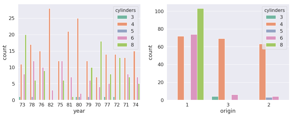
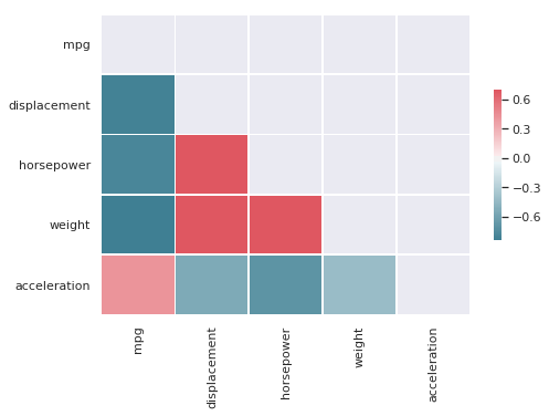
ds.count_plots(data, features.get('catfeatures'))ds.count_plots(data, features.get('catfeatures').copy(), features.get('catfeatures').copy()[0])- A Quick way to find out highly correlated pairs in data, t controls the boundry correlation threshold to filter the features
and generates a sns themed plot
ds.check_correlations(data, features.get("numfeatures"), t=0.8, plot=True)weight and displacement = 0.93282
horsepower and displacement = 0.89726
weight and horsepower = 0.86454
weight and mpg = -0.83174
displacement and mpg = -0.80420
- processOutliers accepts a dataframe of with continuous feature, finds outliers based on IQR range
- for positive/right skew log transformation is applied
- for negative/left skew exponential transformation is applied
- the function returns outliers dataframe and cleaned up dataframe
cleaned_df, outliers = dst.processOutliers(data[features.get('numfeatures')], plot=True, transform=True)____mpg____
lower outlier bound -7.80, upper bound 54.30 ::: number of outliers 0
skew for distribution 0.46
____displacement____
lower outlier bound -242.80, upper bound 609.05 ::: number of outliers 0
skew for distribution 0.72
____horsepower____
lower outlier bound -37.20, upper bound 238.20 ::: number of outliers 6
skew for distribution 1.09
____weight____
lower outlier bound -821.60, upper bound 6653.35 ::: number of outliers 0
skew for distribution 0.53
____acceleration____
lower outlier bound 6.46, upper bound 24.54 ::: number of outliers 2
skew for distribution 0.28
Total Number of outliers: 8
Original shape of data: (398, 5)
New shape of data: (390, 5)
Distribution plots before and Distribution plots After skew adjustment and outlier changes


