A tool that can aggregate information from scientific figures into structured data. For example, extract the functional properities of different variants of opsins - both natual and engineered.
Design an agent that can take in a paper and extract the quantitative results into structured data.
Design an agent that takes in a data scenario and paper/figure examples and then outputs structured data, the data plotted into a figure, and several quantitative questions about the figure with difficulty rankings.
The hope is that the generator could potentially create a dataset to fine-tune the reader by simulating fake experiments and comparing the extrated data to the source data in a loss function. I'm also interested in the possibility of curriculum design such that the generator starts with easy examples and increases diffulty as the reader's performance increases.
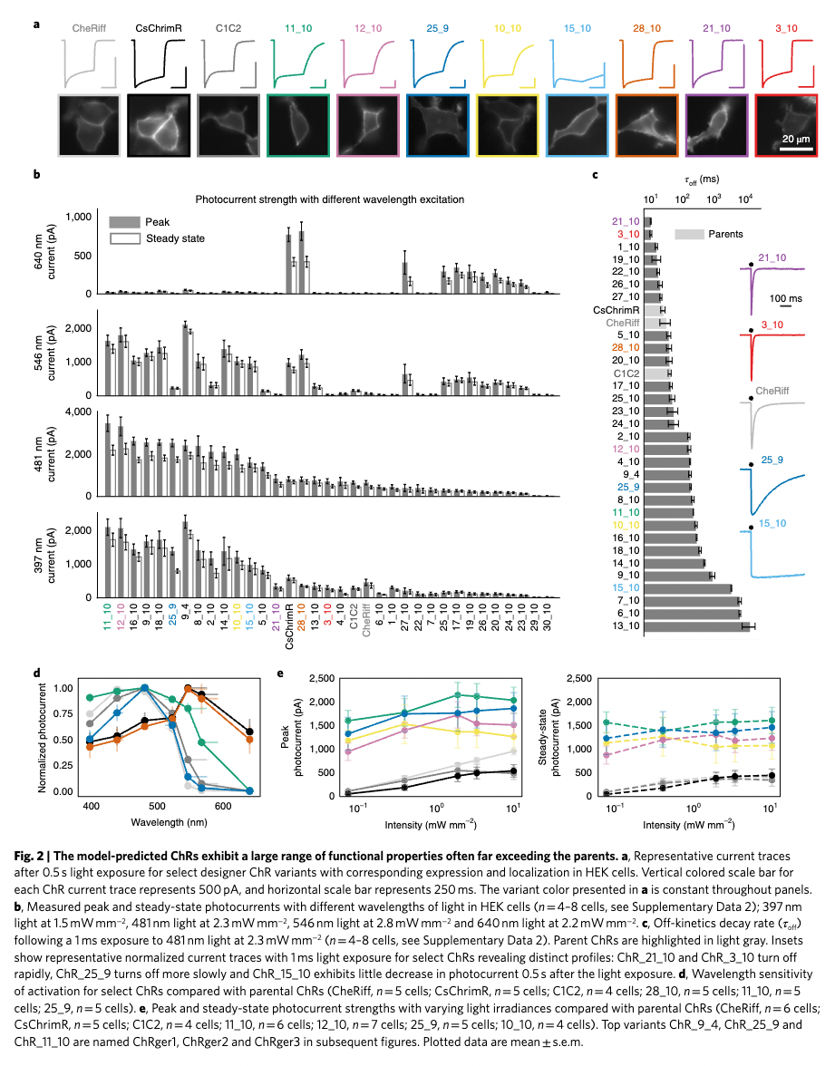
Input Figure (from Machine learning-guided channelrhodopsin engineering enables minimally invasive optogenetics ):
The first step in analyzing a figure is to break down the figure into experiments by plot and to aggregate a legend across the full figure.
Structured Output:
Figure 2
	Legend: [
    CategoryMap(
      type='color',
      values={
        'CheRiff': [0.5, 0.5, 0.5],
        'CsChrimR': [0.0, 0.0, 0.0],
        'C1C2': [0.5, 0.5, 0.5],
        '11_10': [0.0, 1.0, 1.0],
        '12_10': [1.0, 0.0, 1.0],
        '25_9': [0.0, 1.0, 1.0],
        '10_10': [1.0, 1.0, 0.0],
        '15_10': [0.0, 0.0, 1.0],
        '28_10': [1.0, 0.5, 0.0],
        '21_10': [0.5, 0.0, 0.5],
        '3_10': [1.0, 0.0, 0.0]
      }
    )
  ]
	Panel: a

		Plot: Current traces and cell images (plot.text_discrepancies: [])
			independent_variables=[Variable(name='ChR variant', categorical=True, numeric=False), Variable(name='Time', categorical=False, numeric=True)] dependent_variables=[Variable(name='Current', categorical=False, numeric=True), Variable(name='Fluorescence', categorical=False, numeric=True)]
	Panel: b

		Plot: Photocurrent strength with different wavelength excitation (plot.text_discrepancies: [])
			independent_variables=[Variable(name='ChR variant', categorical=True, numeric=False), Variable(name='Wavelength', categorical=True, numeric=True)] dependent_variables=[Variable(name='Photocurrent', categorical=False, numeric=True)]
	Panel: c

		Plot: Off-kinetics decay rate (plot.text_discrepancies: [])
			independent_variables=[Variable(name='ChR variant', categorical=True, numeric=False)] dependent_variables=[Variable(name='τoff', categorical=False, numeric=True)]
		Plot: Representative current traces (plot.text_discrepancies: [])
			independent_variables=[Variable(name='ChR variant', categorical=True, numeric=False), Variable(name='Time', categorical=False, numeric=True)] dependent_variables=[Variable(name='Current', categorical=False, numeric=True)]
	Panel: d

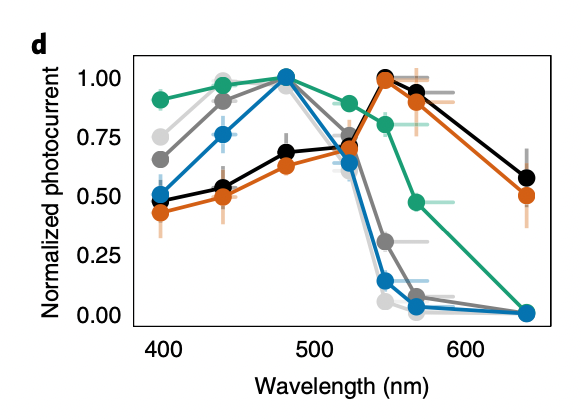
		Plot: Normalized photocurrent vs wavelength (plot.text_discrepancies: [])
			independent_variables=[Variable(name='Wavelength', categorical=False, numeric=True), Variable(name='ChR variant', categorical=True, numeric=False)] dependent_variables=[Variable(name='Normalized photocurrent', categorical=False, numeric=True)]
	Panel: e

		Plot: Peak photocurrent vs intensity (plot.text_discrepancies: [])
			independent_variables=[Variable(name='Light intensity', categorical=False, numeric=True), Variable(name='ChR variant', categorical=True, numeric=False)] dependent_variables=[Variable(name='Peak photocurrent', categorical=False, numeric=True)]
		Plot: Steady-state photocurrent vs intensity (plot.text_discrepancies: [])
			independent_variables=[Variable(name='Light intensity', categorical=False, numeric=True), Variable(name='ChR variant', categorical=True, numeric=False)] dependent_variables=[Variable(name='Steady-state photocurrent', categorical=False, numeric=True)]
Next, we extract more detailed structured information about a particular plot/experiment:
Structured Output:
{
    "independent_variables": [
        {
            "name": "Wavelength",
            "category_maps": [],
            "numeric_axis": {
                "unit": "nm",
                "is_log": false,
                "major_tick_mark_values": [
                    400.0,
                    500.0,
                    600.0
                ]
            }
        },
        {
            "name": "ChR variant",
            "category_maps": [
                {
                    "type": "color",
                    "values": {
                        "CheRiff": [
                            0.5,
                            0.5,
                            0.5
                        ],
                        "CsChrimR": [
                            0.0,
                            0.0,
                            0.0
                        ],
                        "C1C2": [
                            0.7,
                            0.7,
                            0.7
                        ],
                        "11_10": [
                            0.0,
                            0.8,
                            0.8
                        ],
                        "25_9": [
                            0.0,
                            0.5,
                            1.0
                        ],
                        "28_10": [
                            1.0,
                            0.5,
                            0.0
                        ]
                    }
                },
                {
                    "type": "marker",
                    "values": {
                        "CheRiff": "o",
                        "CsChrimR": "o",
                        "C1C2": "o",
                        "11_10": "o",
                        "25_9": "o",
                        "28_10": "o"
                    }
                }
            ],
            "numeric_axis": {
                "unit": "",
                "is_log": false,
                "major_tick_mark_values": []
            }
        }
    ],
    "dependent_variables": [
        {
            "name": "Normalized photocurrent",
            "category_maps": [],
            "numeric_axis": {
                "unit": "",
                "is_log": false,
                "major_tick_mark_values": [
                    0.0,
                    0.25,
                    0.5,
                    0.75,
                    1.0
                ]
            }
        }
    ],
    "parameters": [
        {
            "name": "Light intensity",
            "value": "1.3 mW mm^-2"
        },
        {
            "name": "Light pulse duration",
            "value": "0.5 s"
        }
    ],
    "description": "This experiment measures the normalized photocurrent of different ChR variants across a range of wavelengths.",
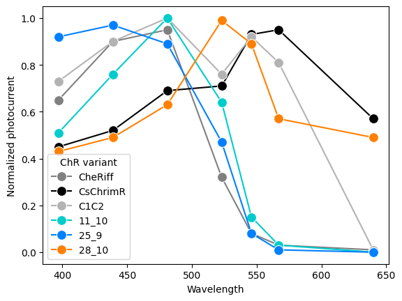
    "result": "The plot shows that different ChR variants have distinct spectral sensitivities. CheRiff and C1C2 have peak sensitivity around 450-500 nm, while CsChrimR and ChR_28_10 are red-shifted with peak sensitivity around 550-600 nm. ChR_11_10 shows a broad activation spectrum, and ChR_25_9 has a narrow activation spectrum peaking around 500 nm.",
    "other_info": "Measurements were taken at seven different wavelengths: 397 \u00b1 3 nm, 439 \u00b1 8 nm, 481 \u00b1 3 nm, 523 \u00b1 6 nm, 546 \u00b1 16 nm, 567 \u00b1 13 nm, and 640 \u00b1 3 nm. The light intensity was matched across wavelengths at 1.3 mW mm^-2.",
    "plot_type": "line plot"
}
Structured output:
[
  NumericVariable(
    name='Wavelength',
    values=[397.0, 439.0, 481.0, 523.0, 546.0, 567.0, 640.0],
    unit='nm'
  ),
  CategoricalVariable(
    name='ChR variant',
    labels=[
      CategoryMap(
        type='color',
        values={
          'CheRiff': [0.5, 0.5, 0.5],
          'CsChrimR': [0.0, 0.0, 0.0],
          'C1C2': [0.7, 0.7, 0.7],
          '11_10': [0.0, 0.8, 0.8],
          '25_9': [0.0, 0.5, 1.0],
          '28_10': [1.0, 0.5, 0.0]
        }
      ),
      CategoryMap(
        type='marker',
        values={
          'CheRiff': 'o',
          'CsChrimR': 'o',
          'C1C2': 'o',
          '11_10': 'o',
          '25_9': 'o',
          '28_10':
          'o'
        }
      )
    ]
  )
]
| INDEX | Wavelength | ChR variant | Normalized photocurrent |
|---|---|---|---|
| 0 | 397.0 | CheRiff | 0.65 |
| 1 | 397.0 | CsChrimR | 0.45 |
| 2 | 397.0 | C1C2 | 0.73 |
| 3 | 397.0 | 11_10 | 0.51 |
| 4 | 397.0 | 25_9 | 0.92 |
| 5 | 397.0 | 28_10 | 0.43 |
| 6 | 439.0 | CheRiff | 0.9 |
| 7 | 439.0 | CsChrimR | 0.52 |
| 8 | 439.0 | C1C2 | 0.9 |
| 9 | 439.0 | 11_10 | 0.76 |
| 10 | 439.0 | 25_9 | 0.97 |
| 11 | 439.0 | 28_10 | 0.49 |
| 12 | 481.0 | CheRiff | 0.95 |
| 13 | 481.0 | CsChrimR | 0.69 |
| 14 | 481.0 | C1C2 | 1.0 |
| 15 | 481.0 | 11_10 | 1.0 |
| 16 | 481.0 | 25_9 | 0.89 |
| 17 | 481.0 | 28_10 | 0.63 |
| 18 | 523.0 | CheRiff | 0.32 |
| 19 | 523.0 | CsChrimR | 0.71 |
| 20 | 523.0 | C1C2 | 0.76 |
| 21 | 523.0 | 11_10 | 0.64 |
| 22 | 523.0 | 25_9 | 0.47 |
| 23 | 523.0 | 28_10 | 0.99 |
| 24 | 546.0 | CheRiff | 0.08 |
| 25 | 546.0 | CsChrimR | 0.93 |
| 26 | 546.0 | C1C2 | 0.92 |
| 27 | 546.0 | 11_10 | 0.15 |
| 28 | 546.0 | 25_9 | 0.08 |
| 29 | 546.0 | 28_10 | 0.89 |
| 30 | 567.0 | CheRiff | 0.03 |
| 31 | 567.0 | CsChrimR | 0.95 |
| 32 | 567.0 | C1C2 | 0.81 |
| 33 | 567.0 | 11_10 | 0.03 |
| 34 | 567.0 | 25_9 | 0.01 |
| 35 | 567.0 | 28_10 | 0.57 |
| 36 | 640.0 | CheRiff | 0.01 |
| 37 | 640.0 | CsChrimR | 0.57 |
| 38 | 640.0 | C1C2 | 0.01 |
| 39 | 640.0 | 11_10 | 0.0 |
| 40 | 640.0 | 25_9 | 0.0 |
| 41 | 640.0 | 28_10 | 0.49 |
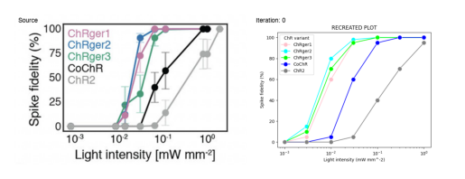
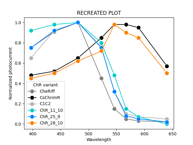
We can replot the data using our extracted values and colors.
| Initial Extraction | Source |
|---|---|
 |
 |
Step 5: Iteratively improve extraction by alternating between a critique substep and revision substep.
| 20 Revision Iterations | Source |
|---|---|
 |
 |
Prompt with both text and example figures.
generator = PlotGenerator(
        storage_dir = "~/dev/plotreader/storage",
    )

generator.generate(
    data_scenario = (
        "Scientists are desigining new opsins by mutating existing ones. " +
        "They then measure the currents produced when exciting with different wavelengths of light. " +
        "They plot comparisons of the different mutants and wild-type as function of these wavelengths."
    ),
    examples_dir='~/dev/plotreader/real_figures/opsins'
)
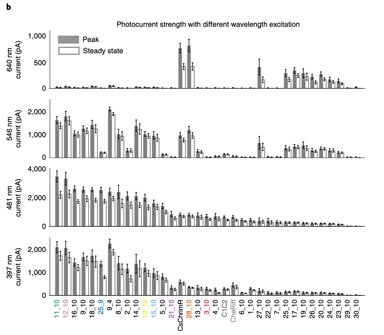
Two of the example figures it was given (from Machine learning-guided channelrhodopsin engineering enables minimally invasive optogenetics).
| Example 1 | Example 2 |
|---|---|
 |
 |
| Example 1 | Example 2 |
|---|---|
 |
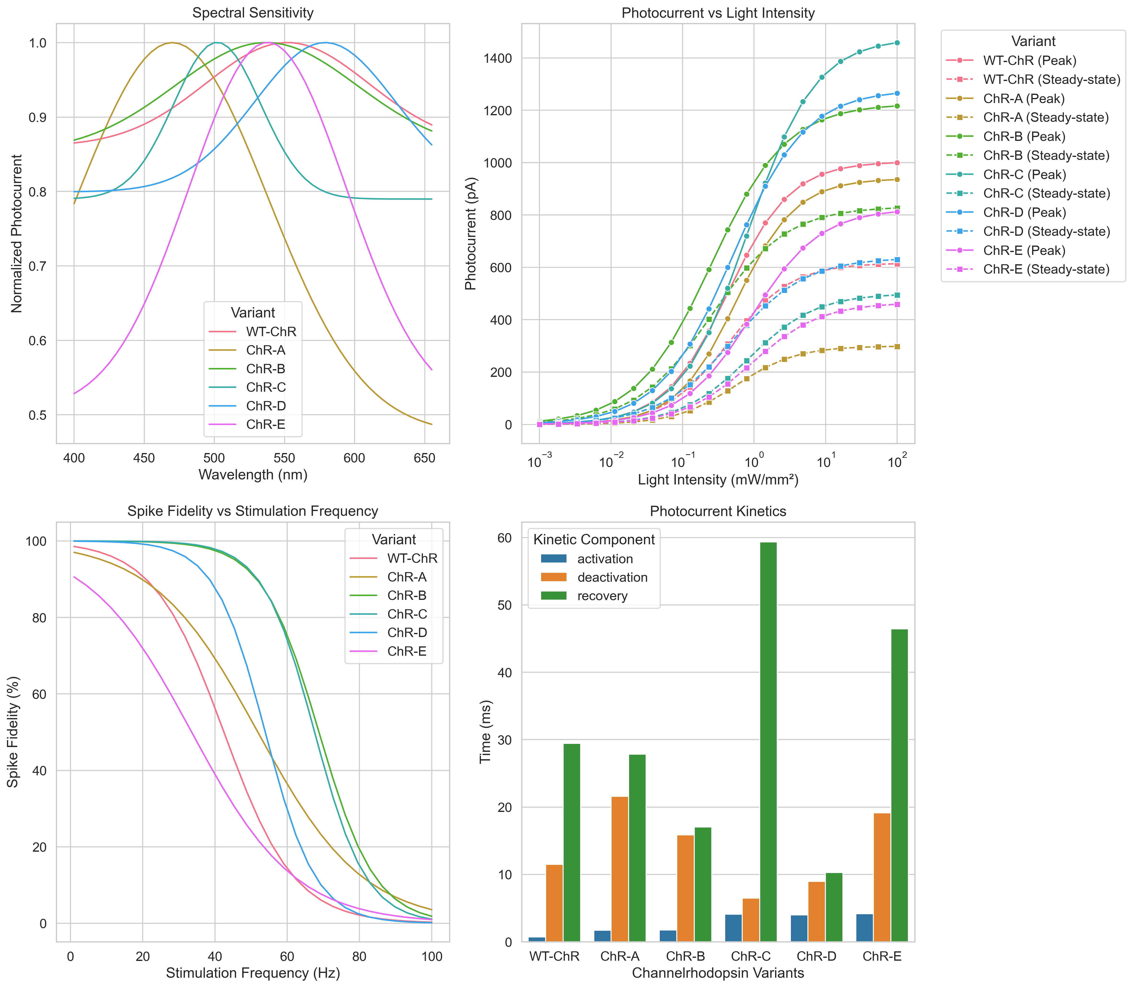 |
The questions were saved into a .json file
[
  {
    "difficulty": "Easy",
    "question": "Which opsin variant shows the highest peak photocurrent at the higher light intensity (0.8 mW mm^-2)?",
    "answer": "ChRger1 shows the highest peak photocurrent at the higher light intensity, with a value of approximately 1500 pA."
  },
  {
    "difficulty": "Medium",
    "question": "Comparing ChR2 and ChRger3, what is the approximate percentage increase in peak photocurrent at the lower light intensity (8 \u00d7 10^-3 mW mm^-2)?",
    "answer": "At the lower light intensity, ChR2 has a peak photocurrent of about 100 pA, while ChRger3 has a peak photocurrent of about 600 pA. The percentage increase is approximately (600 - 100) / 100 * 100 = 500%. ChRger3 shows a 500% increase in peak photocurrent compared to ChR2 at the lower light intensity."
  },
  {
    "difficulty": "Hard",
    "question": "Based on the spectral sensitivity plot, at which wavelength does the difference in normalized photocurrent between ChRger3 and ChR2 appear to be the greatest, and what is the approximate magnitude of this difference?",
    "answer": "The difference in normalized photocurrent between ChRger3 and ChR2 appears to be greatest at around 480-490 nm. At this point, ChRger3 has a normalized photocurrent of about 0.75, while ChR2 has a normalized photocurrent of about 0.55. The magnitude of the difference is approximately 0.75 - 0.55 = 0.2, or a 20% difference in normalized photocurrent."
  }
]Three .csv files were generated that contain the data used to create the figure.
Light intensity response:
| Opsin | Light Intensity (mW mm^-2) | Peak Photocurrent (pA) |
|---|---|---|
| ChR2 | 0.008 | 100 |
| ChR2 | 0.8 | 400 |
| CoChR | 0.008 | 200 |
| CoChR | 0.8 | 900 |
| ChRger1 | 0.008 | 850 |
| ChRger1 | 0.8 | 1500 |
| ChRger2 | 0.008 | 600 |
| ChRger2 | 0.8 | 1400 |
| ChRger3 | 0.008 | 600 |
| ChRger3 | 0.8 | 1300 |
Kinetic estimates:
| Opsin | τoff (ms) |
|---|---|
| ChR2 | 30 |
| CheRiff | 40 |
| C1C2 | 60 |
| ChRger1 | 25 |
| ChRger2 | 35 |
| ChRger3 | 45 |
Spectral Senitivity:
| Wavelength (nm) | Opsin | Normalized Photocurrent |
|---|---|---|
| 400 | ChR2 | 0.036150690739091766 |
| 405 | ChR2 | 0.05259894465789624 |
| 410 | ChR2 | 0.07443440578013699 |
| 415 | ChR2 | 0.1024487550337355 |
| 420 | ChR2 | 0.13714371482751292 |
| 425 | ChR2 | 0.17855885704709237 |
| 430 | ChR2 | 0.22611175977895312 |
| 435 | ChR2 | 0.27848458915645535 |
| 440 | ChR2 | 0.3335918628419484 |
| 445 | ChR2 | 0.38865655282174394 |
| 450 | ChR2 | 0.4404055716042445 |
| 455 | ChR2 | 0.48537329642152754 |
| 460 | ChR2 | 0.520277707898721 |
| 465 | ChR2 | 0.542413914209154 |
| 470 | ChR2 | 0.55 |
| 475 | ChR2 | 0.542413914209154 |
| 480 | ChR2 | 0.520277707898721 |
| 485 | ChR2 | 0.48537329642152754 |
| 490 | ChR2 | 0.4404055716042445 |
| 495 | ChR2 | 0.38865655282174394 |
| 500 | ChR2 | 0.3335918628419484 |
| 505 | ChR2 | 0.27848458915645535 |
| 510 | ChR2 | 0.22611175977895312 |
| 515 | ChR2 | 0.17855885704709237 |
| 520 | ChR2 | 0.13714371482751292 |
| 525 | ChR2 | 0.1024487550337355 |
| 530 | ChR2 | 0.07443440578013699 |
| 535 | ChR2 | 0.05259894465789624 |
| 540 | ChR2 | 0.036150690739091766 |
| 545 | ChR2 | 0.024165313492874083 |
| 550 | ChR2 | 0.01571102543150271 |
| 555 | ChR2 | 0.009934657380879702 |
| 560 | ChR2 | 0.006109948096033269 |
| 565 | ChR2 | 0.003654756205507769 |
| 570 | ChR2 | 0.002126256076710044 |
| 575 | ChR2 | 0.001203120115000587 |
| 580 | ChR2 | 0.0006621229971555117 |
| 585 | ChR2 | 0.0003544089013127345 |
| 590 | ChR2 | 0.00018450444534638154 |
| 595 | ChR2 | 9.342117210877588e-05 |
| 600 | ChR2 | 4.6006590976350145e-05 |
| 400 | CoChR | 0.03668482568419145 |
| 405 | CoChR | 0.05033444988644888 |
| 410 | CoChR | 0.06766764161830635 |
| 415 | CoChR | 0.08913198979252396 |
| 420 | CoChR | 0.11503314949690453 |
| 425 | CoChR | 0.1454619035230741 |
| 430 | CoChR | 0.1802238942989105 |
| 435 | CoChR | 0.2187823688501346 |
| 440 | CoChR | 0.26022506051035105 |
| 445 | CoChR | 0.3032653298563167 |
| 450 | CoChR | 0.34628466210259884 |
| 455 | CoChR | 0.3874187144416247 |
| 460 | CoChR | 0.4246829082841562 |
| 465 | CoChR | 0.4561270384142726 |
| 470 | CoChR | 0.48000272064273886 |
| 475 | CoChR | 0.4949239016893669 |
| 480 | CoChR | 0.5 |
| 485 | CoChR | 0.4949239016893669 |
| 490 | CoChR | 0.48000272064273886 |
| 495 | CoChR | 0.4561270384142726 |
| 500 | CoChR | 0.4246829082841562 |
| 505 | CoChR | 0.3874187144416247 |
| 510 | CoChR | 0.34628466210259884 |
| 515 | CoChR | 0.3032653298563167 |
| 520 | CoChR | 0.26022506051035105 |
| 525 | CoChR | 0.2187823688501346 |
| 530 | CoChR | 0.1802238942989105 |
| 535 | CoChR | 0.1454619035230741 |
| 540 | CoChR | 0.11503314949690453 |
| 545 | CoChR | 0.08913198979252396 |
| 550 | CoChR | 0.06766764161830635 |
| 555 | CoChR | 0.05033444988644888 |
| 560 | CoChR | 0.03668482568419145 |
| 565 | CoChR | 0.02619657053491279 |
| 570 | CoChR | 0.018329020976689005 |
| 575 | CoChR | 0.012565244492637209 |
| 580 | CoChR | 0.008439942074394954 |
| 585 | CoChR | 0.005554498269121153 |
| 590 | CoChR | 0.0035816822354596085 |
| 595 | CoChR | 0.0022629039333833595 |
| 600 | CoChR | 0.0014008190174242421 |
| 400 | ChRger3 | 0.10150146242745953 |
| 405 | ChRger3 | 0.1293162179203146 |
| 410 | ChRger3 | 0.1621988751224155 |
| 415 | ChRger3 | 0.2002888764197575 |
| 420 | ChRger3 | 0.2434893505187623 |
| 425 | ChRger3 | 0.2914185956342731 |
| 430 | ChRger3 | 0.3433750213287107 |
| 435 | ChRger3 | 0.3983219932765089 |
| 440 | ChRger3 | 0.45489799478447507 |
| 445 | ChRger3 | 0.5114555633927611 |
| 450 | ChRger3 | 0.5661297014917555 |
| 455 | ChRger3 | 0.6169331717989985 |
| 460 | ChRger3 | 0.6618726769384466 |
| 465 | ChRger3 | 0.6990768692696456 |
| 470 | ChRger3 | 0.7269249258572581 |
| 475 | ChRger3 | 0.7441634536951827 |
| 480 | ChRger3 | 0.75 |
| 485 | ChRger3 | 0.7441634536951827 |
| 490 | ChRger3 | 0.7269249258572581 |
| 495 | ChRger3 | 0.6990768692696456 |
| 500 | ChRger3 | 0.6618726769384466 |
| 505 | ChRger3 | 0.6169331717989985 |
| 510 | ChRger3 | 0.5661297014917555 |
| 515 | ChRger3 | 0.5114555633927611 |
| 520 | ChRger3 | 0.45489799478447507 |
| 525 | ChRger3 | 0.3983219932765089 |
| 530 | ChRger3 | 0.3433750213287107 |
| 535 | ChRger3 | 0.2914185956342731 |
| 540 | ChRger3 | 0.2434893505187623 |
| 545 | ChRger3 | 0.2002888764197575 |
| 550 | ChRger3 | 0.1621988751224155 |
| 555 | ChRger3 | 0.1293162179203146 |
| 560 | ChRger3 | 0.10150146242745953 |
| 565 | ChRger3 | 0.07843425096675109 |
| 570 | ChRger3 | 0.05966963153867076 |
| 575 | ChRger3 | 0.044690489071489564 |
| 580 | ChRger3 | 0.032952700217555565 |
| 585 | ChRger3 | 0.023921095021617825 |
| 590 | ChRger3 | 0.017095635662709257 |
| 595 | ChRger3 | 0.012028281956512912 |
| 600 | ChRger3 | 0.008331747403681729 |
