Using Low Dose CT data from AAPM
You can find details about Low Dose CT Grand Challenge from this Official Website.
You can download data set(~7.6GB) from data link.
Download the data.zip and extract. After you can find data folder, place data folder in main project directory. Main project directory must be configured as follow.
│  .gitignore
│  dataset.py
│  inference.ipynb
│  inference_unet.ipynb
│  make_noise_target.ipynb
│  model.py
│  README.md
│  train.ipynb
│  train_unet.ipynb
│  utils.py
│
├─data
│  ├─test
│  │  ├─fd
│  │  │      1.npy
│  │  │      2.npy
│  │  │      3.npy
|  |  |      ...
│  │  │
│  │  └─qd
│  │          1.npy
│  │          2.npy
│  │          3.npy
|  |          ...
│  │
│  └─train
│      ├─fd
│      │      1.npy
│      │      2.npy
│      │      3.npy
|      |      ...
│      │
│      └─qd
│              1.npy
│              2.npy
│              3.npy
|              ...
│
└─images_README
        0041.png
        0052.png
        0059.png
        ...
- The goal of this challenge and our project is to de-noise low dose(quarter dose) CT Image to get high dose(full dose) CT Image.
Inside the data folder you will find two sub folder qd and fd each representing quarter dose and full dose.
Quarter dose corresponds to low dose and full dose corresponds to high dose.
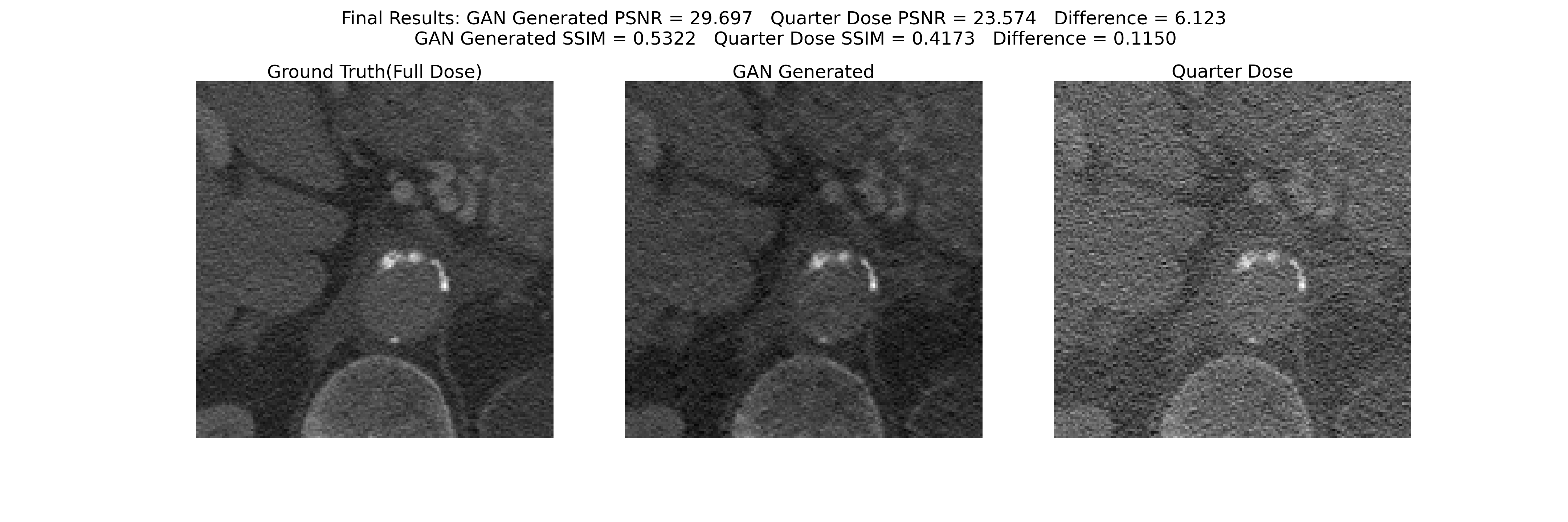
Typical data look like below.
You can see the noise in quarter dose image compared to full dose image.
For clarity, I also included center cropped image below.
For the generator, we used U-net based generator.
For the discriminator, we used 70X70 PatchGAN.
We used Adam optimizer with a batch size of 8, total epoch was 80 epochs. Initial learning rate was 0.0002. First half the total epoch, I remained same learning rate and linearly decay the learning rate to zero over the next remaining epochs.
Below is the PSNR(Peak Signal to Noise Ratio) between Ground truth(full dose CT image) with U-net generator generated image.
For the other loss values during training, you can find graph image inside images_README folder.
- PSNR
- Average PSNR between Test set Quarter Dose and Test set Full Dose: 26.9565dB
- Average PSNR between Test set Full Dose and U-net Generator generated image: 34.4406dB
- PSNR gain:
7.4842dB
- SSIM
- Average SSIM between Test set Quarter Dose and Test set Full Dose: 0.6988
- Average SSIM between Test set Full Dose and U-net Generator generated image: 0.8598
- SSIM gain:
0.1610
(PSNR, SSIM with respect to Full Dose)
- Full Image (512X512 size)
- Center Cropped Image (150X150 size)
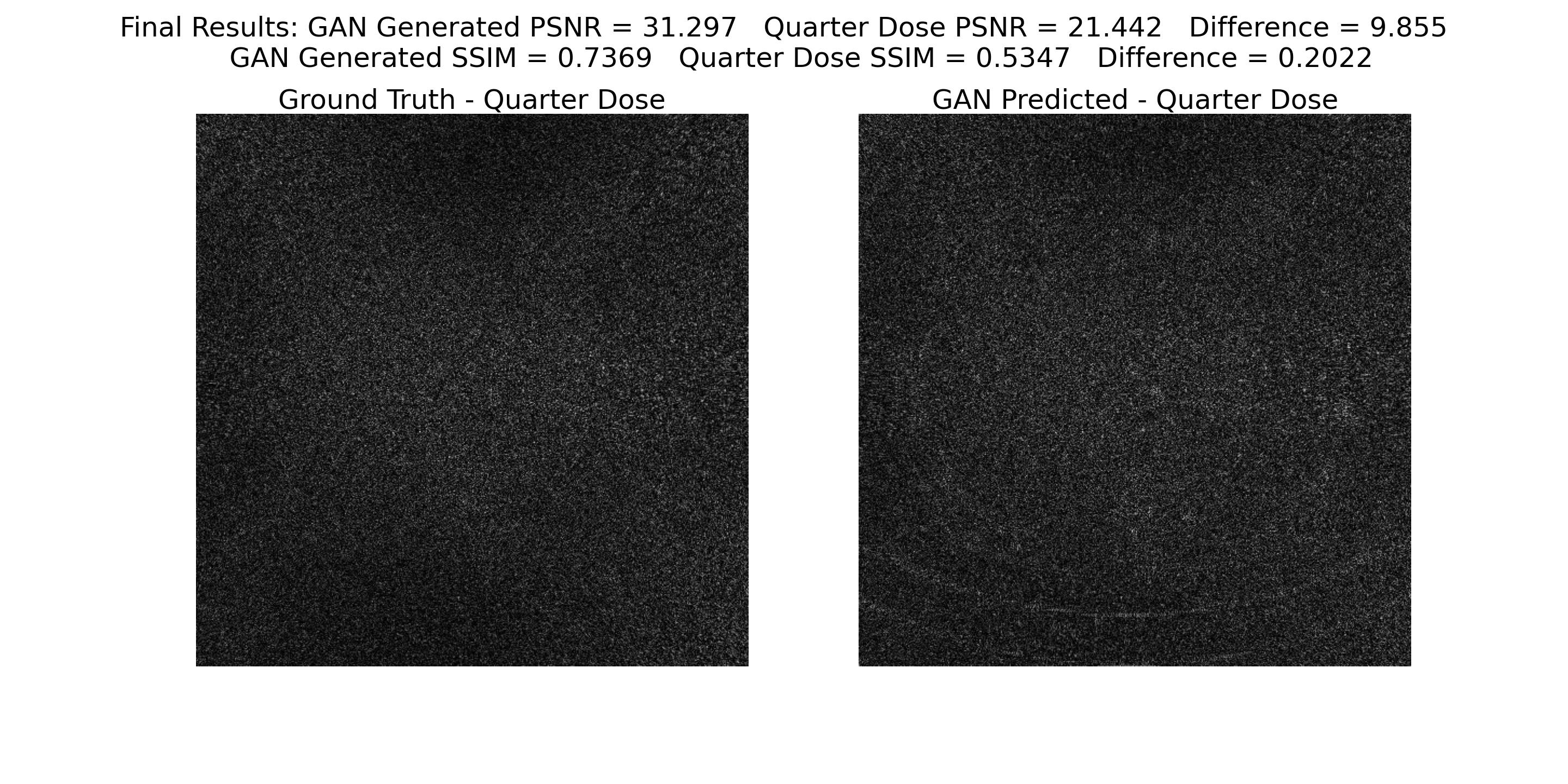
- Noise Comparison
Left image is the noise(difference between full dose and quarter dose) and the right image is the noise(difference between generated signal and quarter dose) eliminated by Cycle GAN. You can see that Cycle GAN properly eliminates noise from quarter dose signal.
- torch (1.11.0)
- torchvision (0.12.0)
- torchmetrics
- torchsummary
- tqdm
- PIL
- numpy
- matplotlib
- tensorboard (optional)
- Download data.zip and place
datafolder, containingtestandtrainsubfolder, inside the main project directory.
- No data preprocessing is used. We will use raw signal data from
dataas input to model. - The only processing used is
torchvision.transforms.RandomCropto downsize image from 512X512 to 256X256.
- Run
train.ipynb. Model will be saved underfinal_resultfolder. - Run
tensorboard --logdir ./runsto monitor training.
- Run
inference.ipynb. You can get PSNR and SSIM value for your trained model. - Inside
inference.ipynbyou can findplot_resultfunction. It will generate image like the one in Result section.cropparameter will center crop the image to given size.saveparameter will save image under the folderfinal_imageorfinal_image_centerif you usecropparameter. plot_reult_diffgenerate image like the one in Noise Comparison. Parameters are same asplot_resultfunction. It will save image under the folderfinal_image_difforfinal_image_diff_centerif you usecropparameter.
To use pretrained model, download final_result.zip and place the unzipped folders (Discriminator_A, GAN_FD_to_QD...) under final_result folder. And go to 3. Inference.
Main project directory must be configured as follow in order to use pretrained model.
│  .gitignore
│  dataset.py
│  inference.ipynb
│  inference_unet.ipynb
│  make_noise_target.ipynb
│  model.py
│  README.md
│  train.ipynb
│  train_unet.ipynb
│  utils.py
│
├─data
│  ├─test
│  │  ├─fd
│  │  │       ...
│  │  └─qd
│  │          ...
│  │
│  └─train
│      ├─fd
│      │      ...
│      └─qd
│             ...
│
├─final_result
│  │  history.pkl
│  │
│  ├─Discriminator_A
│  │      Disc_A.pt
│  │
│  ├─Discriminator_B
│  │      Disc_B.pt
│  │
│  ├─GAN_FD_to_QD
│  │      GAN.pt
│  │
│  └─GAN_QD_to_FD
│          GAN.pt
│
└─images_README
        0041.png
        0052.png
        ...
We used U-net as a baseline model for comparison with our cycle GAN model. We selected U-net as a baseline model since U-net is frequently used model for de-noising task.
This section is instruction for training baseline model (U-net) and for providing comparison with cycle GAN model.
- Run
train_unet.ipynb. Model will be saved underfinal_result_denoising_unetfolder. - Run
tensorboard --logdir ./runsto monitor training.
This step includes comparison with cycle GAN model. So in order to execute this step, you must have trained cycle GAN model in your directory. (final_result folder must be in your main project folder)
- Run
inference_unet.ipynb. You can get PSNR and SSIM value for your trained model. - Inside
inference_unet.ipynbyou can findplot_resultfunction. This is the same function introduced before. plot_result_comparisonfunction compares the de-noised result between baseline model and cycle GAN generator model.cropparameter will center crop the image to given size.saveparameter will save image under the folderfinal_image_comparison_with_noiseorfinal_image_center_comparison_with_noiseif you usecropparameter.
To use pretrained baseline model, download final_result_denoising_unet.zip and place the unzipped folder final_result_denoising_unet under main project directory. And go to 2. Inference.
Main project directory must be configured as follow in order to use pretrained baseline model.
│  .gitignore
│  dataset.py
│  inference.ipynb
│  inference_unet.ipynb
│  model.py
│  README.md
│  train.ipynb
│  train_unet.ipynb
│  utils.py
│
├─data
│  ├─test
│  │  ├─fd
│  │  │       ...
│  │  └─qd
│  │          ...
│  │
│  └─train
│      ├─fd
│      │      ...
│      └─qd
│             ...
│
├─final_result
│  │  history.pkl
│  │
│  ├─Discriminator_A
│  │      Disc_A.pt
│  │
│  ├─Discriminator_B
│  │      Disc_B.pt
│  │
│  ├─GAN_FD_to_QD
│  │      GAN.pt
│  │
│  └─GAN_QD_to_FD
│          GAN.pt
│
├─final_result_denoising_unet
│      denoising_unet.pt
│      history.pkl
│
└─images_README
        0041.png
        0052.png
        ...
We present Loss function used for generator and discriminator.
We follow the notation given in the original paper. Check the image below.
- Generator Loss Function
- Discriminator Loss Function
We tested for various U-net depth(7 layer, 8 layer, 9 layer) where layer represents one concatenation, so our final model presented above is 8 layer U-net Generator.
| # of layers | PSNR Gain(dB) | Center Cropped image(350X350) PSNR Gain(dB) | SSIM Gain | Center Cropped image(350X350) SSIM Gain | Noise PSNR |
|---|---|---|---|---|---|
| 7 layer | 6.6638 | 4.8668 | 0.1484 | 0.1187 | 19.8380 |
| 8 layer | 7.4842 | 5.2259 | 0.1610 | 0.1236 | 19.9271 |
| 9 layer | 7.3119 | 4.6682 | 0.1555 | 0.1048 | 19.6466 |
For 7 layer, 8 layer U-net generator, we used RandomCrop with 256X256 size and trained with total 80 epochs. For 9 layer U-net generator 256X256 input is unavailable so we used full size image(512X512 size) and trained for 30 epochs. As you can see our best model was achevied using 8 layer U-net.


