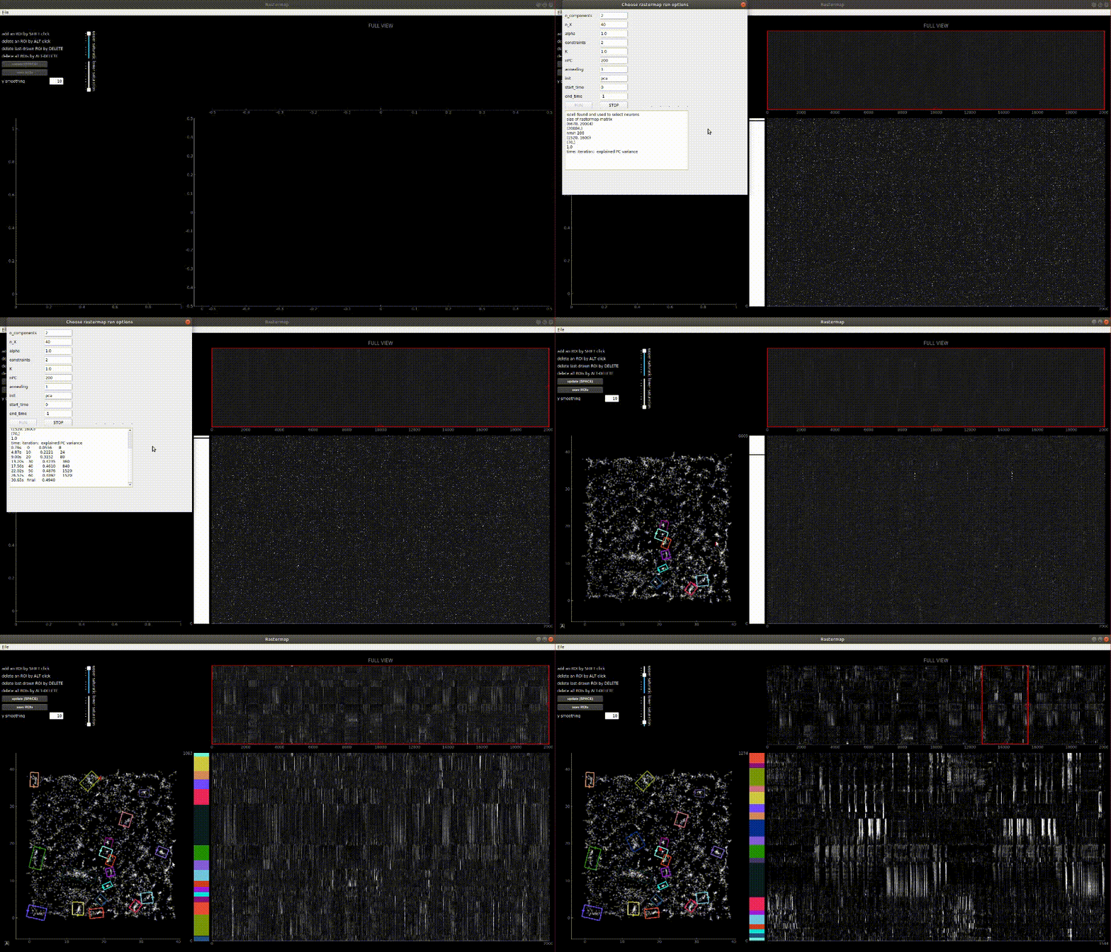
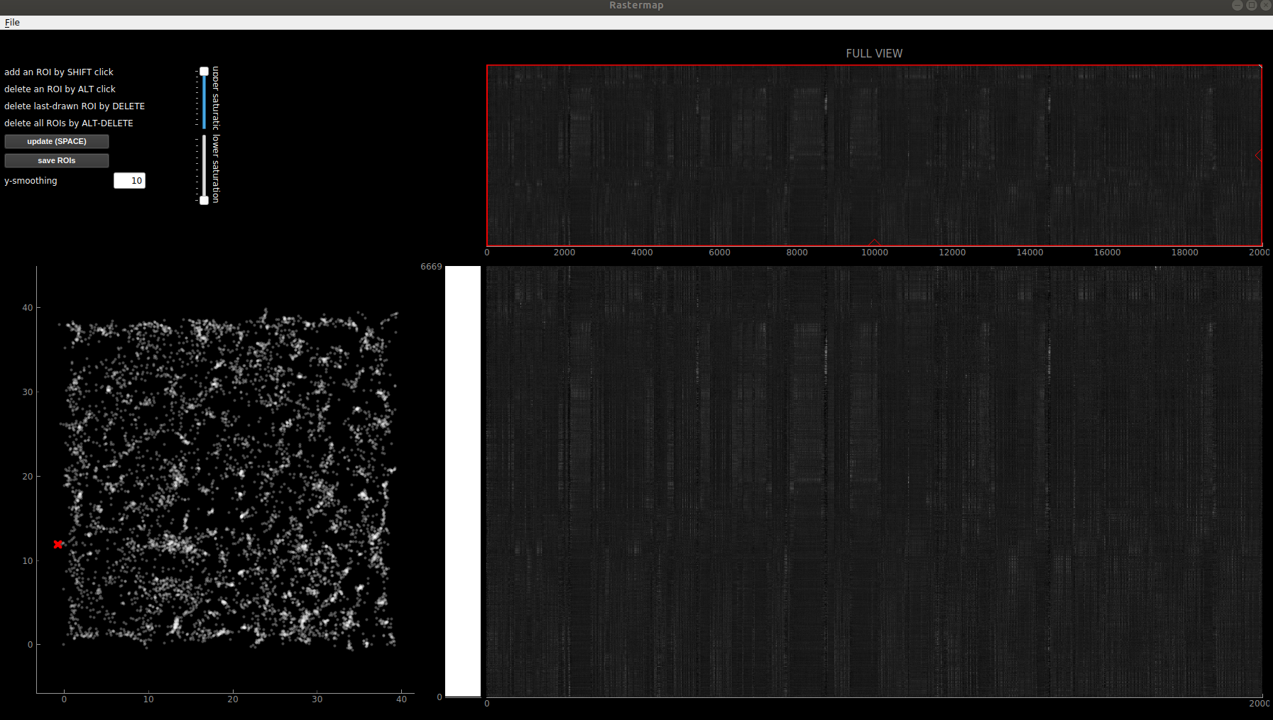
This algorithm computes a 1D or 2D embedding of neural activity. It assumes that the spike matrix S is neurons by timepoints. We have a python 3 and a matlab implementation, and have a GUI for running it in the python implementation. See the demos for jupyter notebooks using it, and some example data. We also have a guided tutorial integrating suite2p, rastermap, and facemap in an attempt to understand visual cortical responses.
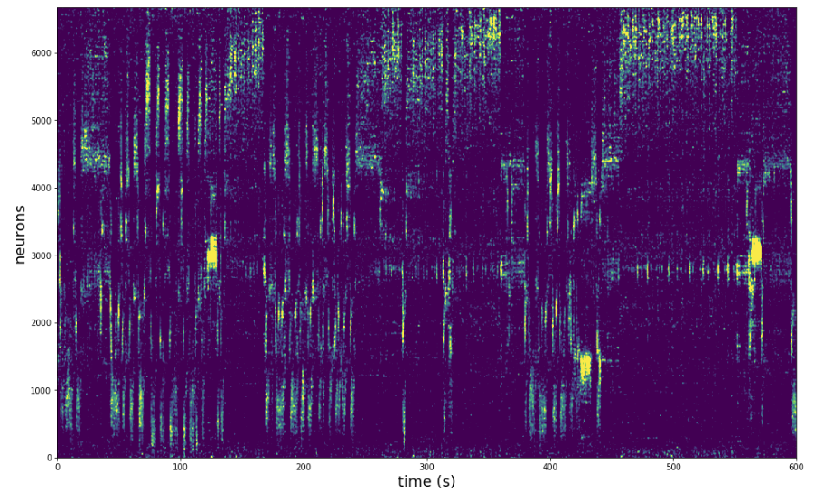
Here is what the output looks like for a segment of a mesoscope recording (2.5Hz sampling rate) (sorted in neural space, but not time space):
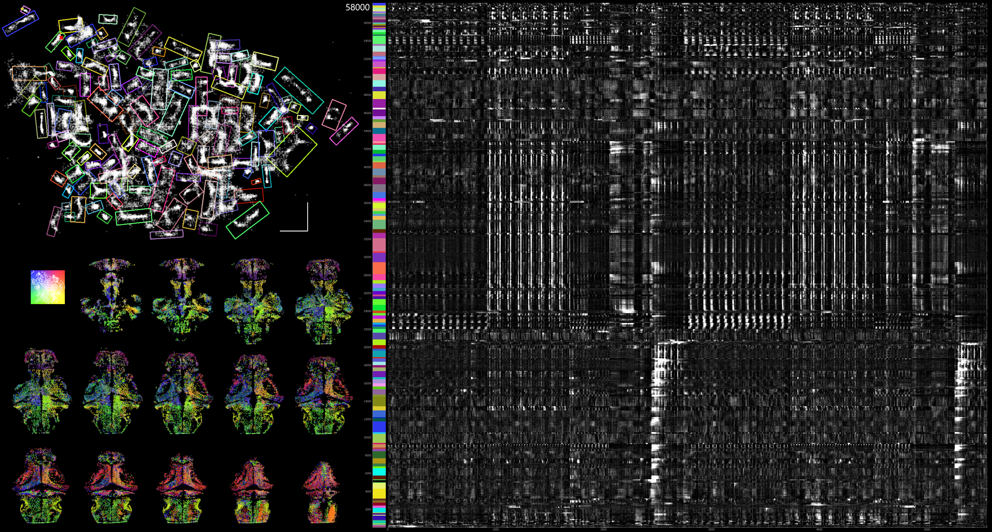
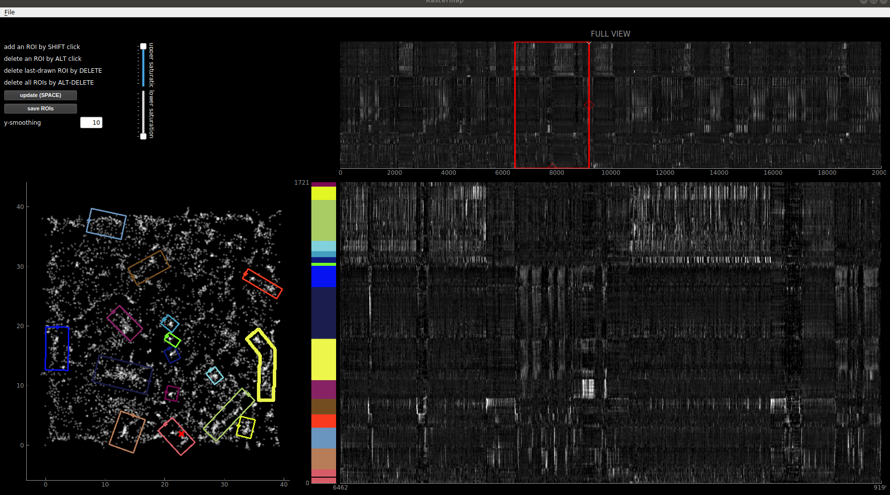
Here is what the output looks like for a recording of 64,000 neurons in a larval zebrafish (data here, thanks to Chen, Mu, Hu, Kuan et al / Ahrens lab for sharing!). The upper left plot is the 2D embedding with boxes around clusters (which the user draws in the GUI). The plot on the right shows the activity of the clusters. The lower left plot is a Z-stack of the neurons in the tissue, colored according to their 2D position in the Rastermap embedding.
Install an Anaconda distribution of Python -- Choose Python 3.x and your operating system. Note you might need to use an anaconda prompt if you did not add anaconda to the path.
- Download the
environment.ymlfile from the repository. You can do this by cloning the repository, or copy-pasting the text from the file into a text document on your local computer. - Open an anaconda prompt / command prompt with
condafor python 3 in the path - Change directories to where the
environment.ymlis and runconda env create -f environment.yml - To activate this new environment, run
conda activate rastermap - You should see
(rastermap)on the left side of the terminal line. Now runpython -m rastermapand you're all set.
If you have an older rastermap environment you can remove it with conda env remove -n rastermap before creating a new one.
Note you will always have to run conda activate rastermap before you run suite2p. Conda ensures pyqt and numba run correctly and quickly on your machine. If you want to run jupyter notebooks in this environment, then also conda install jupyter.
... Or you can pip install the package and the pyqt5 requirements (not as recommended):
pip install PyQt5 PyQt5.sip
pip install rastermap
And then open the GUI with
python -m rastermap
You can download the github folder and run the command inside the folder
This package was written for Python 3 and relies on the awesomeness of numpy, scipy, PyQt5, PyQt5.sip and pyqtgraph. You can pip install or conda install all of these packages. If having issues with PyQt5, then make an Anaconda environment and try to install within it.
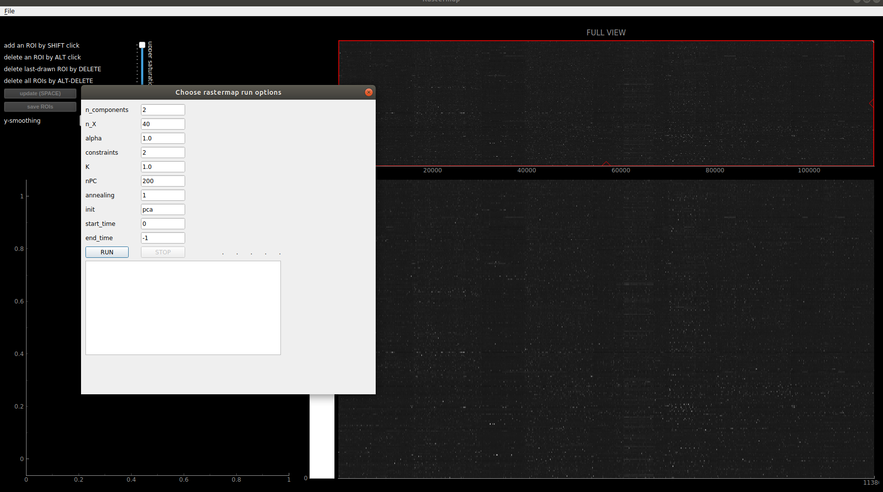
Save your data into an npy file that is just a matrix that is neurons x features. Then "Load data matrix" and choose this file. Next click "Run embedding algorithm" and run with TWO components if you want to visualize it in the GUI. See the parameters section to learn about the parameters.
The embedding will pop up in the GUI when it's done running, and save the embedding in the same folder as your data matrix with the name "embedding.npy".
To draw ROIs around points in the GUI, you draw multiple line segments and then resize them. The neurons' activity traces then show up on the right side of the GUI sorted along this "line axis" that you've drawn. To start drawing a line, hold down SHIFT and click for the first point, and keep clicking to make more segments. To end the segment, click WITHOUT holding down SHIFT. Then resize the box and click again to complete the ROI. Do NOT hold down the mouse, that will just drag you all over the place :) To update the plot on the right with the selected cells on the left, hit the SPACE key. You can delete the last ROI with the DELETE button, or delete a specific ROI by clicking inside that ROI and holding down ALT. You can save the ROIs you've drawn with the "save ROIs" button. They will save along with the embedding so you can reload the file with the "Load processed data" option.
How to load the embedding outside the GUI:
import numpy as np
model = np.load('embedding.npy')
model = model.dict()
y = model['embedding'] # neurons x n_components
NOTE: If you are using suite2p "spks.npy", then the GUI will automatically use the "iscell.npy" file in the same folder to subsample your recording with the chosen cells.
rastermap can be run the same way as the T-SNE embedding algorithm or other algorithms in scikit-learn. Rastermap is a class which has functions fit, fit_transform, and transform (embeds new points into original embedding).
(input should be n_samples x n_features like t-sne, etc)
# >> from github <<
import sys
sys.path.append('/media/carsen/DATA2/Github/rastermap/rastermap/')
from mapping import Rastermap

# >> from pip <<
from rastermap import Rastermap

model = Rastermap(n_components=1, n_X=30, nPC=200, init='pca')

# fit does not return anything, it adds attributes to model
# attributes: embedding, u, s, v, isort1

model.fit(sp)
plt.imshow(sp[model.isort1, :])

# fit_transform returns embedding (upsampled cluster identities)
embedding = model.fit_transform(sp)

# transform can be used on new samples with the same number of features as sp
embed2 = model.transform(sp2)
Rastermap first takes the specified PCs of the data, and then embeds them into n_X clusters. It returns upsampled cluster identities (n_X x upsamp). Clusters are also computed across Y (n_Y) and smoothed, to help with fitting.
- n_components : int, optional (default: 2) dimension of the embedding space
- n_X : int, optional (default: 40) size of the grid on which the Fourier modes are rasterized
- nPC : nparray, int, optional (default: 400) how many of the top PCs to use during optimization
- alpha : float, optional (default: 1.0) exponent of the power law enforced on component n as: 1/(K+n)^alpha
- K : float, optional (default: 1.0) additive offset of the power law enforced on component n as: 1/(K+n)^alpha
- init : initialization of algorithm (default: 'pca') can use 'pca', 'random', or a matrix n_samples x n_components
Rastermap model has the following attributes after running 'fit':
- embedding : array-like, shape (n_samples, n_components) Stores the embedding vectors.
- u,sv,v : singular value decomposition of data S, potentially with smoothing
- isort1 : sorting along first dimension (n_samples) of matrix
- cmap : correlation of each item with all locations in the embedding map (before upsampling)
- A : PC coefficients of each Fourier mode
This package was written for Python 3 and relies on numpy and scipy. The Python3.x Anaconda distributions will contain all the dependencies.
The matlab version requires Matlab 2016a or later. If you want to use the GPU acceleration (useGPU=1), then you need an NVIDIA GPU and the Parallel Computing Toolbox. Otherwise, I don't think it requires any additional toolboxes, but please let me know if it does in the issues.
The matlab code needs to be cleaned up but the main function to call is mapTmap.m. This function is used in the example script loadFromPython.m (loads suite2p outputs, requires npy-matlab).
