Easy Creation of GnuPlot Scripts from C++

What is it?

A simple C++17 library that allows easy creation and execution of gnuplot scripts. These scripts will embed their data and can be replayed/modified later.

The library depends on {fmt} library.

I use it when I want to plot some data with a minimal effort when I develop stuff in C++.

For the moment the library is only tested under Linux (it should also works under Windows but I have not checked yet).

News

[2020-10-20 Tue]
- Version v1.1.0!
- some compilation warning fixes
- a new Data_Array_2 class
[2020-01-18 Sat 09:17]
- Version v1.0.0 release!
- More documentation
- Fix a bug in export_as(…,path/output_filename): the path was ignored
[2020-01-09 Thu 22:46]
- Added Data_Supervised class and associated example (see Density plot in Example section)
- Code cleaning (no breaking change!)
- Tagged as v0.2.0 (v1.0.0 gets closer :-) )
[2019-12-09 Mon 18:34]
Added SVG, TGIF, PNGCairo and PDFCairo export formats. Tagged as v0.0.3.
[2019-12-08 Sun 20:21]
Some minor fixes + doc concerning Global_Config logger methods. Tagged as v0.0.2
[2019-12-08 Sun 11:21]
Initial version. Tagged as v0.0.1

Contributors

Guillaume Jacquenot: Travis CI

Installation

The library currently uses the meson build system.

If you are not familiar with meson, the compilation procedure is as follows:

git clone https://github.com/vincent-picaud/GnuPlotScripting.git
cd GnuPlotScripting/
meson build
cd build
ninja test

Examples can then be found in the build/examples/ directory.

If you want to install the package:

ninja install

Note that you can define custom installation path, at the beginning of the compilation procedure, use:

meson --prefix=/install_path/ build

instead of meson build.

Examples

Plot and fit data

#include "GnuPlotScripting/GnuPlotScripting.hpp"

#include <iostream>
#include <vector>

using namespace GnuPlotScripting;

// From: https://www.cs.hmc.edu/~vrable/gnuplot/using-gnuplot.html

int
main()
{
  std::vector<double> time, angle, stdvar;

  time = {0.0,  1.0,  2.1,  3.1,  4.2,  5.2,  6.2,  7.2,  8.2,  9.1,  10.0, 11.0, 12.0,
          12.9, 13.8, 14.9, 15.9, 17.0, 17.9, 18.9, 20.0, 21.0, 22.0, 23.0, 24.0, 25.0,
          26.0, 27.0, 28.0, 29.0, 30.0, 31.0, 32.0, 32.9, 33.8, 34.7, 35.7, 36.6, 37.7};

  angle = {-14.7, 8.6,  28.8, 46.7, 47.4, 36.5, 37.0, 5.1,  -11.2, -22.4, -35.5, -33.6, -21.1,
           -15.0, -1.6, 19.5, 27.5, 32.6, 27.5, 20.2, 13.8, -1.3,  -24.5, -25.0, -25.0, -20.2,
           -9.9,  5.8,  14.7, 21.8, 29.8, 21.4, 24.6, 25.8, 0.6,   -16.6, -24.0, -24.6, -19.8};

  stdvar = {3.6, 3.6, 3.0, 3.4, 3.5, 3.4, 10.3, 3.4,  3.4, 3.5, 3.6, 3.9, 3.9,
            4.2, 2.7, 3.2, 2.8, 3.5, 2.7, 3.3,  3.4,  4.2, 6.7, 3.3, 3.1, 3.6,
            3.2, 3.2, 3.0, 3.5, 2.7, 4.1, 2.7,  12.0, 2.9, 3.2, 3.7, 3.8, 3.5};

  Script_File script("plot.gp");

  Data_Vector data(
      time, angle, stdvar);  // <- you can stack as many vector/valarray etc.. as you want
                             //    only size() and operator[] are required.

  script.free_form("set title 'Cavendish Data'");
  script.free_form("set xlabel 'Time (s)'");
  script.free_form("set ylabel 'Angle (mrad)'");
  script.free_form("set grid");
  script.free_form("plot {} with yerrorbars notitle", data);
  script.free_form("replot {} u 1:2 with lines title '{}'", data, "raw data");
  script.free_form("theta(t) = theta0 + a * exp(-t / tau) * sin(2 * pi * t / T + phi)");
  script.free_form("fit theta(x) {} using 1:2:3 via a, tau, phi, T, theta0", data);
  script.free_form("replot theta(x) lw {} lc {} title 'best-fit curve'", 2, 4);
  script.export_as(PNG(), "plot");
}

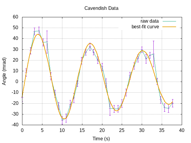
It generates this figure:

Note: the generated plot.gp gnutplot script embeds the data and you can replay it whenever you want:

gnuplot plot.pg -

Ascii matrix data

#include "GnuPlotScripting/GnuPlotScripting.hpp"

#include <iostream>

using namespace GnuPlotScripting;

// Example from: https://stackoverflow.com/a/27049991/2001017
// Also see: https://stackoverflow.com/q/32458753/2001017
//
int
main()
{
  Data_Ascii data(
      "0.00 0.65 0.65 0.25\n"
      "0.25 0.00 0.75 0.25\n"
      "0.50 0.60 0.00 0.25\n"
      "0.75 0.25 0.10 0.00\n");

  Script_File script("matrix.gp");

  script.free_form("set autoscale fix");
  script.free_form("set cbrange [-1:1]");
  script.free_form("unset colorbox");
  script.free_form("unset key");
  script.free_form(
      "plot {} matrix using 1:2:3 with image, '' matrix using "
      "1:2:(sprintf('%.2f', $3)) with labels font ',16'",
      data);
  script.export_as(PNG(), "matrix");
  script.export_as(EPSLATEX().set_standalone(true), "matrix");
}

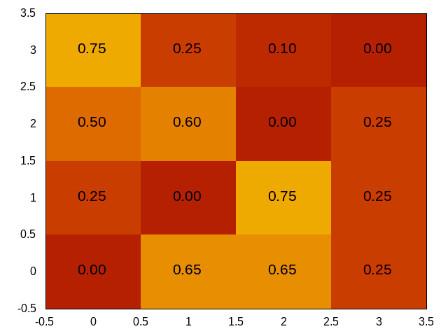
It generates this figure:

It also generates a standalone matrix.tex file you can process with pdflatex matrix.tex to get a monochrome matrix.pdf file. If you want colorized pdf simply use:

EPSLATEX().set_standalone(true).set_color(true)

(NEW) Matrix data

You can also use the Array_2 container to temporary store your data

#include "GnuPlotScripting/array_2.hpp"
#include "GnuPlotScripting/GnuPlotScripting.hpp"

#include <iostream>

using namespace GnuPlotScripting;

int
main()
{
  const double X = 2, Y = 2;
  const std::size_t I = 100, J = 120;

  const auto f = [=](const std::size_t i, const std::size_t j) {
    const double x = (2 * i / double(I - 1) - 1) * X;
    const double y = (2 * j / double(J - 1) - 1) * Y;

    return exp(-x * x - y * y);
  };

  Array_2 array_2(I, J, f);

  Data_Array_2 data(array_2);

  Script_File script("array_2.gp");

  script.free_form("set autoscale fix");
  script.free_form("plot {} matrix using 1:2:3 with image", data);
  script.export_as(PNG(), "array_2");
}

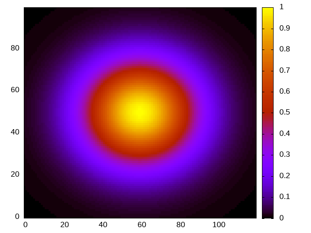
It generates this figure:

Histogram

#include "GnuPlotScripting/GnuPlotScripting.hpp"

#include <iostream>
#include <random>

using namespace GnuPlotScripting;

// Example from:
// https://stackoverflow.com/a/7454274/2001017
//
template <typename T>
void
gnuplot_histogram(Script& script,
                  const std::vector<T>& data,
                  const size_t n_bin,
                  const typename std::vector<T>::value_type min,
                  const typename std::vector<T>::value_type max)
{
  assert(max > min);
  assert(n_bin > 0);

  Data_Vector gnuplot_data(data);

  const double width = (max - min) / n_bin;
  script.free_form("width={}", width);
  script.free_form("set title 'Histogram min={}, max={}, Δbin={}, #bins={}, #sample={}'",
                   min,
                   max,
                   width,
                   n_bin,
                   data.size());
  script.free_form("hist(x,width)=width*floor(x/width)+width/2.0");
  script.free_form("set boxwidth width*0.9");
  script.free_form("set style fill solid 0.5");
  script.free_form("plot {} u (hist($1,width)):(1.0) smooth freq w boxes notitle", gnuplot_data);
}

int
main()
{
  std::random_device rd;
  std::mt19937 gen(rd());
  const double a = 2, b = 1;
  std::gamma_distribution<> distribution(a, b);

  std::vector<double> data(10000);
  for (auto& data_i : data) data_i = distribution(gen);

  Script_File script("histogram.gp");

  gnuplot_histogram(script, data, 100, 0, 3);

  script.export_as(PNG(), "histogram");
}

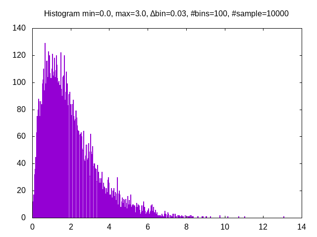
The generated figure is:

Graph

#include "GnuPlotScripting/GnuPlotScripting.hpp"

#include <iostream>

using namespace GnuPlotScripting;

// Example from the "Gnuplot in Action" book
int
main()
{
  Data_Ascii data(
      "-1 -1 0    # A\n"
      "-1  1 0    # B\n"
      " 1  0 0    # C\n"
      " 0  0 1.75 # D\n"
      "\n\n"
      "-1 -1 0   -1 1 0     \n"
      "-1 -1 0    1 0 0     \n"
      "-1 -1 0    0 0 1.750 \n"
      "-1  1 0    1 0 0     \n"
      "-1  1 0    0 0 1.75  \n"
      " 1  0 0    0 0 1.75  \n");

  Script_File script_a("graph_3D.gp");

  script_a.free_form("unset border");
  script_a.free_form("unset tics");
  script_a.free_form("unset key");
  script_a.free_form("set view 75,35");
  script_a.free_form("splot {} index 0 with points pointtype 7 pointsize 3", data);
  script_a.free_form("replot {} index 1 u 1:2:3:($4-$1):($5-$2):($6-$3) with vectors nohead", data);
  script_a.free_form("pause -1");

  Script_File script_b("graph_2D.gp");

  script_b.free_form("unset border");
  script_b.free_form("unset tics");
  script_b.free_form("unset key");
  script_b.free_form("plot {} index 0 with points pointtype 7 pointsize 3", data);
  script_b.free_form("replot {} index 1 u 1:2:($4-$1):($5-$2) with vectors nohead", data);
  script_b.export_as(PNG(), "graph");
}

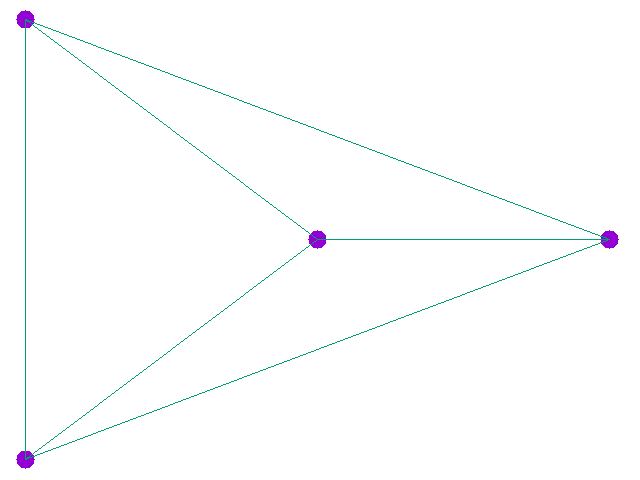
It generates this figure:

but also an active gnuplot 3D figure you can rotate etc…

Density plot

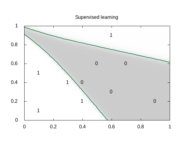
This demo shows how to use the Data_Supervised class.

#include "GnuPlotScripting/GnuPlotScripting.hpp"

#include <array>
#include <iostream>

using namespace GnuPlotScripting;

std::array<double, 10> X_1 = {0.1, 0.3, 0.1, 0.6, 0.4, 0.6, 0.5, 0.9, 0.4, 0.7};
std::array<double, 10> X_2 = {0.1, 0.4, 0.5, 0.9, 0.2, 0.3, 0.6, 0.2, 0.4, 0.6};
std::array<int, 10> Y      = {1, 1, 1, 1, 1, 0, 0, 0, 0, 0};

int
main()
{
  Data_Supervised data(Y, X_1, X_2);

  Script_File script("density_plot.gp");

  script.free_form("set title 'Supervised learning'");

  script.free_form("set pm3d map interpolate 2,2");
  script.free_form("set palette model RGB defined ( 0 'gray80', 1 'white' )");
  script.free_form("set contour base");
  script.free_form("set cntrparam levels discrete 0.5");
  script.free_form("unset colorbox");  // no palette

  // CAVEAT: for contour use pm3d and not image
  script.free_form(
      "splot 'density_plot_data.txt' u ($1/60):($2/60):3 matrix with pm3d lw 2 notitle");

  for (size_t i = 0; i < data.index_size(); i++)
  {
    // CAVEAT: to prevent
    //         <<warning: Cannot contour non grid data. Please use "set dgrid3d">>
    //         do not forget "nocontour"
    script.free_form(
        "replot {0} index {1} u 1:2:3 with points pt '{1}' ps 2 notitle nocontour", data, i);
  }

  script.export_as(PNG(), "density_plot");

  return EXIT_SUCCESS;
}

Generated figure:

Pipe example

Instead of creating a file, we can create a pipe with popen() to directly send data to gnuplot.

#include "GnuPlotScripting/GnuPlotScripting.hpp"

#include <chrono>
#include <iostream>
#include <thread>
#include <utility>  // std::pair
#include <vector>

using namespace GnuPlotScripting;

int
main()
{
  // AFAIK one has to replot all data at each iteration
  //
  std::vector<std::pair<size_t, double>> data;

  Script_Pipe pipe(Script_Pipe_Mode_Enum::Not_Persistent);

  pipe.free_form("set xlabel 'iterations'");

  for (size_t i = 0; i < 100; i++)
  {
    data.push_back({i, 1 / (i + 1.)});

    pipe.free_form("plot '-' using 1:2 with lines t \"residue\" ");
    for (const auto& data_i : data)
    {
      pipe.free_form("{} {}", data_i.first, data_i.second);
    }
    pipe.free_form("e");
    pipe.flush();

    std::this_thread::sleep_for(std::chrono::milliseconds(50));
  }
}

Supported export formats

This example silently exports a basic plot in all supported formats:

#include "GnuPlotScripting/GnuPlotScripting.hpp"

#include <iostream>

using namespace GnuPlotScripting;

int
main()
{
  Script_File script("available_export_formats.gp", Script_File_Mode_Enum::Silent);

  script.free_form("plot sin(x) t 'sin(x)'");

  script.export_as(PNG(), "available_export_formats");
  script.export_as(EPSLATEX().set_standalone(true), "available_export_formats");
  script.export_as(SVG(), "available_export_formats");
  script.export_as(TGIF(), "available_export_formats");
  script.export_as(PNGCairo(), "available_export_formats_cairo");
  script.export_as(PNGCairo().set_color(false), "available_export_formats_cairo_nocolor");
  script.export_as(PDFCairo(), "available_export_formats_pdfcairo");
}

Global config demonstration

This last example shows how to use Global_Config.

#include "GnuPlotScripting/GnuPlotScripting.hpp"

#include <iostream>

using namespace GnuPlotScripting;

int
main()
{
  global_config().set_logger(
      [](const char *const msg) { std::cerr << "====> My logger " << msg << std::endl; });
  // If you want to remove logger:  global_config().set_logger();
  // If you want to restore the default one: global_config().set_default_logger();

  // If you want to globally overwrite Script_File_Mode_Enum to Persistent, do:
  global_config().set_script_file_mode(Script_File_Mode_Enum::Persistent);

  for (size_t i = 1; i < 5; i++)
  {
    Script_File script(fmt::format("script_{}.gp", i), Script_File_Mode_Enum::Silent);

    script.free_form("plot sin({0}*x) t 'sin({0}*x)'", i);
  }

  // To stop overwriting local choice:
  global_config().set_script_file_mode();

  // Now this will silently run scripts
  for (size_t i = 1; i < 5; i++)
  {
    Script_File script(fmt::format("script_{}.gp", i), Script_File_Mode_Enum::Silent);

    script.free_form("plot sin({0}*x) t 'sin({0}*x)'", i);
  }
}

Documentation

The library is quite simple and there is only 3 things you must know:

Data_XXX are classes to store your data
Script_XXX are script classes to write your scripts
global_config() returns a Global_Config object used to define global options.

Data classes

Data classes store data that is embedded into the generated gnuplot scripts. These classes internally use an uuid that insures that data is embedded only once. By example, when you write:

script.free_form("plot {} u 1:2",data);
script.free_form("replot {} u 1:3",data);
script.free_form("replot {} u 1:4",data);

data is copied only once into the script file.

`Data_Ascii`

The most basic Data classe is the Data_Ascii one. It directly uses data defined by a std::string. By example:

Data_Ascii data(
    "0.00 0.65 0.65 0.25\n"
    "0.25 0.00 0.75 0.25\n"
    "0.50 0.60 0.00 0.25\n"
    "0.75 0.25 0.10 0.00\n");

Note: it is really easy to define your own Data class. By example Data_Ascii code is as simple as:

class Data_Ascii final : public Data
{
 public:
  Data_Ascii(const std::string& data) : Data(data) {}
};

(NEW) `Data_Array_2`

Data to plot is defined using an basic two-dimensional array container, Array_2.

Array_2 array_2(row_size,column_size);

// fill component: array_2(i,j)= ...

Data_Array_2 data(array_2);

// plot data

`Data_Vector`

Creates columns of data from std::vector, std::valarray… In fact only the size() method and the operator[] operator are used and you can use any object defining these two methods. By example:

std::vector<double> v1(10);
std::vector<int> v2(10);
std::valarray<double> v3(10);
// ...
Data_Vector data(v1,v2,v3);

`Data_Supervised`

The Data_Supervised class is similar to the Data_Vector except that it uses and extra category vector. It can be used to plot points associated to a supervised learning task. By example:

std::array<double, 10> X_1 = {0.1, 0.3, 0.1, 0.6, 0.4, 0.6, 0.5, 0.9, 0.4, 0.7};  // X_1 feature
std::array<double, 10> X_2 = {0.1, 0.4, 0.5, 0.9, 0.2, 0.3, 0.6, 0.2, 0.4, 0.6};  // X_2 feature
std::array<int, 10> Y      = {1, 1, 1, 1, 1, 0, 0, 0, 0, 0};                      // category (=label)

Data_Supervised data(Y, X_1, X_2); // note: the category vector Y is always the _first_ argument

std::cout << data.data();

Note: as AFAK it is not possible to directly plot points with symbols retrieved from the the Y column (see SO how-set-point-type-from-data-in-gnuplot), hence the Data_Supervised class sorts and groups the sample according to their categories. By example the previous code prints:

Creating these groups allows to use the gnuplot index keyword to plot all points associated to a given category. By example:

replot "$data_uuid" index i u 1:2:3 with points; # plot points of category i

Also note that when data is embedded, the Y category column is the last one. The rational is that for:

Data_Supervised data_a(Y, X_1, X_2); 
Data_Vector data_b(X_1, X_2);

then in both cases, X_1 column index is 1 and X_2 column index is 2.

Script classes

There are two script classes:

Script_File creates a file to store the script.
Script_Pipe creates a pipe to push data directly to GnuPlot, in that case no file is created.

They inherits from the Script base class that provides the following methods:

template <typename... ARGS>
Script& free_form(ARGS&&... args);

Script& export_as(const Export_As& export_as, const std::filesystem::path& output);

void flush();

free_form allows you to write free form using the fmt library, by example:

script.free_form("plot '{}' u {}:{}","data_file.dat",1,2);

flush() forces buffer to be flushed
export_as() generates script code to export the figure in the given format, by example:

script.export_as(EPSLATEX().set_standalone(true),"filename");

Note:

the right extension for filename is automatically added (here this would be .tex).
currently supported formats are PNG, EPSLATEX, SVG, TGIF, PNGCairo and PDFCairo.

`Script_File` class

The only relevant part is the constructor:

Script_File(const std::filesystem::path& filename,
            Script_File_Mode_Enum script_file_mode = Script_File_Mode_Enum::Persistent);

Filename is the gnuplot script file name (you are free to use the file extension you want, on my side I use the .gp extension).
script_file_mode is important as it defines what happens at destruction time
- Script_File_Mode_Enum::None does nothing
- Script_File_Mode_Enum::Silent silently runs GnuPlot (this will generate your exported figures)
- Script_File_Mode_Enum::Persistent runs GnuPlot in persistent mode, it will generates your figures and left a window opened that allows you to see the result. This is only an opened window and not an active gnuplot session (you cannot interact with the plot).

Note: to get an active GnuPlot session, you can replay your script with:

gnuplot filename.gp -

(note the final ‘-‘, see GnuPlot documentation for further details).

Another possibility is to add a pause in your gnuplot script:

script.free_form("pause -1");

`Script_Pipe` class

Here instead of writing into a file, we open a pipe with popen. This allows you to directly command GnuPlot during your code execution. Note that this is only a unidirectional channel.

The constructor is:

Script_Pipe(Script_Pipe_Mode_Enum script_pipe_mode = Script_Pipe_Mode_Enum::Persistent);

as for Script_File class, script_pipe_mode defines what happens at destruction time:

Script_Pipe_Mode_Enum::Not_Persistent does not keep an opened window
Script_Pipe_Mode_Enum::Persistent keeps an opened, but inactive, window

Global_Config class

This class allows you to define or overwrite globally some options

const char* gnuplot_exe() const;
Global_Config& set_gnuplot_exe(const char* const gnuplot_executable);

Global_Config& set_logger();          // removes logger
Global_Config& set_default_logger();  // reuses default one
Global_Config& set_logger(const std::function<void(const char* const msg)>& f);  // defines your own
bool has_logger() const;
Global_Config& set_log_message(const char* const msg);

Global_Config& set_script_file_mode(
    Script_File_Mode_Enum mode);        // globally overwrite local 'script_file_mode'
Global_Config& set_script_file_mode();  // stop overwriting local 'script_file_mode'
std::optional<Script_File_Mode_Enum> script_file_mode() const;

set/gnuplot_exe() functions allow you to define GnuPlot executable filename, by default this is gnuplot or gnuplot.exe for windows.
set/logger() functions allow you to stop or redirect logs, by example:

global_config().set_logger([](const char *const msg) {
  std::cerr << "====> My logger " << msg << std::endl;
});

set_script_file_mode() functions are more interesting as they allow you to overwrite globally what happens at Script_File destruction time. A typical use case is as follows:
Imagine that your code silently generates a lot of scripts:

for (size_t i = 1; i < 5; i++)
{
  Script_File script(fmt::format("script_{}.gp", i), Script_File_Mode_Enum::Silent);

  script.free_form("plot sin({0}*x) t 'sin({0}*x)'", i);
}

However at debug time, you want to force visualization to see what happens. In that case you simply have to add

global_config().set_script_file_mode(Script_File_Mode_Enum::Persistent);

before

for (size_t i = 1; i < 5; i++)
{
  ...
}

This will force all Script_File to use Script_File_Mode_Enum::Persistent

References

GnuPlot official page
GnuPlot in Action a very well written book
www.gnuplotting.org a lot of great examples
GnuPlot not so Frequently Asked Questions
Wikipedia the free encyclopedia…

FAQ

-> your question here

Name		Name	Last commit message	Last commit date
Latest commit History 145 Commits
examples		examples
figures		figures
src		src
subprojects		subprojects
test		test
.clang-format		.clang-format
.dockerignore		.dockerignore
.gitignore		.gitignore
.travis.yml		.travis.yml
Dockerfile		Dockerfile
LICENSE		LICENSE
Makefile_travis		Makefile_travis
README.org		README.org
meson.build		meson.build

Provide feedback

Saved searches

Use saved searches to filter your results more quickly

Repository files navigation

Easy Creation of GnuPlot Scripts from C++

Table of contents

What is it?

News

Contributors

Installation

Examples

Plot and fit data

Ascii matrix data

(NEW) Matrix data

Histogram

Graph

Density plot

Pipe example

Supported export formats

Global config demonstration

Documentation

Data classes

`Data_Ascii`

(NEW) `Data_Array_2`

`Data_Vector`

`Data_Supervised`

Script classes

`Script_File` class

`Script_Pipe` class

Global_Config class

References

FAQ

About

Releases

Packages

Contributors 3

Languages

License

vincent-picaud/GnuPlotScripting

Folders and files

Latest commit

History

Repository files navigation

Easy Creation of GnuPlot Scripts from C++

Table of contents

What is it?

News

Contributors

Installation

Examples

Plot and fit data

Ascii matrix data

(NEW) Matrix data

Histogram

Graph

Density plot

Pipe example

Supported export formats

Global config demonstration

Documentation

Data classes

Data_Ascii

(NEW) Data_Array_2

Data_Vector

Data_Supervised

Script classes

Script_File class

Script_Pipe class

Global_Config class

References

FAQ

About

Topics

Resources

License

Stars

Watchers

Forks

Releases

Packages 0

Contributors 3

Languages

`Data_Ascii`

(NEW) `Data_Array_2`

`Data_Vector`

`Data_Supervised`

`Script_File` class

`Script_Pipe` class

Packages